81 bricks array

This is example illustrates multiple aspects of Solfec-1.0 functionality and serves as a validation test. It is also included with TR1. The input files for this example are located in the solfec/examples/81array directory. These are:

• README – a text based summary of the problem

• 81array.py – array excitation analysis input file

• 81fbi.py – fuel brick impact test input file

• 81postp.py – post–processing script for the 81array.py input deck

• 81array[*].inp files – ABAQUS input decks used by 81array.py

• 81fbi[*].inp files – ABAQUS input decks used by 81fbi.py

• 81array[*]base.pikle.gz files – saved reduced POD base files used by 81array.py and 81fbi.py

• FB[*].csv files – experimental results curves used by 81postp.py

• ts81.py.bz2 file – compressed time history of a seisimic excitation signal used by 81array.py

Fig. 71 Example 81array: experimental setup of the experiment.

The experiment behind this example comes from the context of the civil nuclear power generation in the UK. A series of dynamic tests were carried out by National Nuclear Corporation in 1985 as part of the seismic endorsement of the Heysham II / Torness AGR * core design. These tests used an array of 81 graphite bricks as shown in Fig. 71, consisting of alternating ‘fuel’ and ‘interstitial’ bricks. The array was mounted in a rigid frame on a shaker table. The boundary frame was driven in the horizontal plane with synthesized seismic or swept–sine input motions in either one or both axes simultaneously. Measurements were taken of the resulting velocities of certain bricks in the array (determined from accelerometer data) and also of the forces within the keying system (using load cells built into some components). Some details of the experimental setup has been described in 1 and 2. We note, that this example is also called the “81 bricks array”, or simply the “81 array”, because the total number of unconstrained fuel and interstitial bricks is 81.

Fig. 72 Example 81array: meshed model (base mesh).

In the current demonstration we bypass many of the details of our mechanical model. The ultimate aim is modeling the entire AGR core (\(\sim5\text{K}\) fuel bricks), hence we are in the search for the lowest possible resolution model. We are going to demonstrate some results for two mesh densities: denoted as a “basic mesh” and a “fine mesh”, cf. Table 32. The basic meshed model is presented in Fig. 72. As in the experiment all bodies are vertically restrained so that they move in a frictionless manner in the horizontal plane. Since the behavior of the assembly is essentially two dimensional the number of elements along the height is kept to minimum. In Fig. 73 one can see that the number of elements used in the horizontal brick sections is also small. For fuel brick meshes the error in the lowest eigenmodes corresponding to planar squeezing is below 35% (as compared with finer meshes), which we tentatively accept in the quest for a lowest possible resolution model.

Error

Unable to execute python code at 81array.rst:68:

[Errno 2] No such file or directory: ‘solfec/examples/81array/81module_fbi.png’

Fig. 73 Example 81array: array module closeup (left: base mesh) and the binary impact test (right: fine mesh).

Table 32 Example 81array: base and fine mesh statistics. There are 61 fuel bricks, 60 interstitial bricks, and 100 loose keys in each case.

			Fuel brick	Interstitial brick	Loose key	Model total
BC	base mesh	DOFs	432	456	24	56112
	fine mesh		1512	456	24	121992
BC–RO	base mesh		64	64	24	10144
	fine mesh		64	64	24	10144

The following material parameters were assumed for the graphite used in the experiment: 1.18E10Pa for Young’s modulus, 0.21 for Poisson’s ratio, and for mass density 1688kg/\(\mbox{m}^{3}\), 1637kg/\(\mbox{m}^{3}\), 1740kg/\(\mbox{m}^{3}\) for respectively fuel bricks, interstitial bricks and loose keys (the mass densities were tuned to obtain the total brick weights reported in the experiment). The coefficient of Coulomb’s friction was assumed 0.1. Among several simple impact tests performed in the preliminary experimental work, a binary impact between fuel bricks was Fig. 73 (right). A range of relative input velocities was used (5–35 cm/s) for which the ratio of the output velocity to the input velocity remained consistently in the area of 0.9. It should be noted that due to geometrical setup, this particular type of impact is not present in our full array model. We then have two independent experiments, which we try to validate simultaneously.

We use three families of models: solely rigid (RG), body co-rotational (BC), and reduced order (BC–RO). In all cases the time step is 0.0001s. Co–rotated displacements from the BC simulation were sampled at 0.02s intervals and together with the 6 algebraically generated rigid modes, for each distinct mesh instance, served as an input for the Python modred package, to produce POD bases for the BC-RO approach: 64 modes were used for both the fuel and the interstitial bricks. The loose keys were modeled as single elements based on the co–rotated BC approach. For the deformable models we used damping \(\eta=\mbox{1E-7}\), which, for the finer mesh, roughly reproduced the required macroscopic velocity restitution of 0.9 for the binary impact test from Fig. 71 (right): restitution of 0.91 was produced by the BC approach, and 0.86 by BC–RO. For the basic mesh, the reproduced coefficient of restitution was 0.85 for the BC approach, and 0.82 for BC–RO. In case of the rigid body model the impact restitution was zero, resulting in a totally passive response.

In the initial validation of the entire array model we aimed at reproducing a swept–sine constant amplitude acceleration test. In the experiment the array was subject to a 3s 3Hz settling dwell at start, followed by a 3Hz to 10Hz sweep with 0.1Hz/s buildup rate and constant amplitude of 0.3g, all this amounting to the total duration of 72s. The sweep direction was aligned with one of the sides of the array. Linear velocity histories of the centre points of several bricks were recorded at 50Hz. Magnitudes of these velocities were then averaged using 0.1Hz window and plotted as time series normalized by the corresponding magnitudes of the input velocity.

The input acceleration signal produces a smoothly decaying envelope of displacement, which given a fixed amount of clearance between bricks, initially builds up their “rattling” interactions and then passes a threshold beyond which interactions cease. Initially the displacements are much larger than the clearance and the entire array is swept back and forth. When the boundary displacements reach the level of the clearance (few mm) the kinetic energy starts being injected into higher modes of the system. This builds up a peak in the velocity response. When the input displacements fall below the clearance distance the bricks disengage and there is a drop in the velocity response.

Fig. 74 Example 81array: frequency histories of normalized output velocity magnitudes. EXP is the experiment. BC–base and BC–fine denote the body co–rotational formulation using respectively the base and the fine mesh.

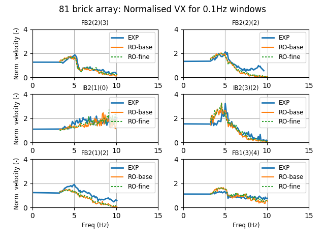
Fig. 75 Example 81array: frequency histories of normalized output velocity magnitudes. EXP is the experiment. RO–base and RO–fine denote the reduced order formulation using respectively the base and the fine mesh.

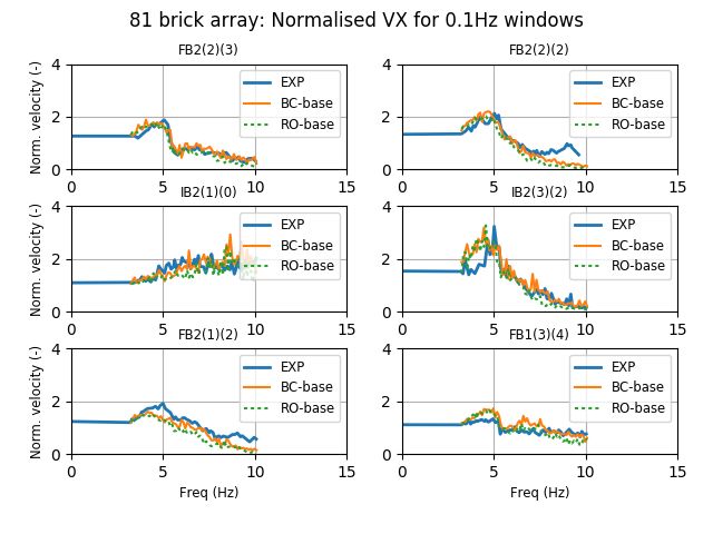
Fig. 76 Example 81array: frequency histories of normalized output velocity magnitudes. EXP is the experiment. BC–base and RO–base are respectively the BC and the BC–RO formulations, both using the base mesh.

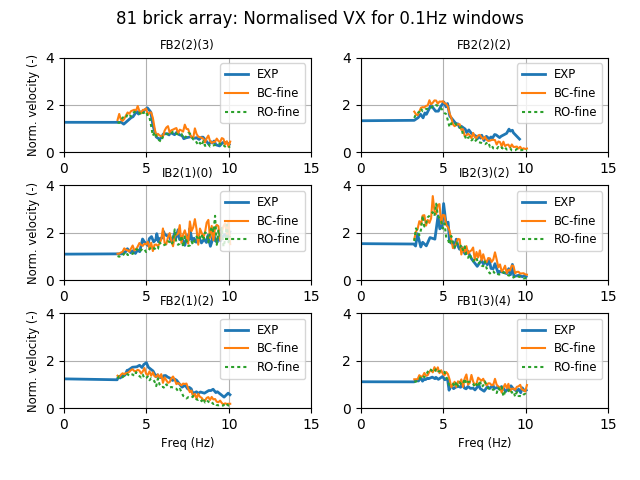
Fig. 77 Example 81array: frequency histories of normalized output velocity magnitudes. EXP is the experiment. BC–fine and RO–fine are respectively the BC and the BC–RO formulations, both using the fine mesh.

Fig. 74 – Fig. 77 show time histories of normalized output velocity magnitudes for selected fuel and interstitial bricks, compared with those obtained in the experiment. One can see that relatively good agreement is obtained for all combinations of base and fine FE meshes combined with the body co–rotational (BC) and reduced order BC–RO (dented as RO in the figures) formulations. The best overall match seems to be obtained in case of the BC–fine model: combining the body co–rotational formulation (BC) and the fine mesh (where only the fuel bricks are refined). This is specifically visible in Fig. 74 and Fig. 77 where the performance of the BC–fine model for the FB2(2)(2) fuel brick is better than of the BC–base and RO–fine models. There seems to be some correlation between the ability to reproduce the 0.9 binary impact velocity restitution from the experiment, and the ability to match most of the experimental curves in Fig. 74 – Fig. 77. On the other hand, Fig. 78 compares the performance of the BC–base approach with that of the purely rigid body model (RG). Clearly, the rigid body approach is not able to reproduce the experimentally observed peaks.

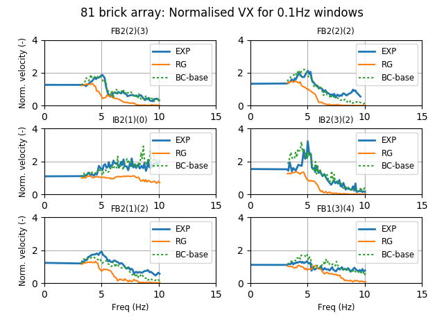
Fig. 78 Example 81array: frequency histories of normalized output velocity magnitudes. EXP is the experiment. RG and BC–base are respectively the rigid body and the body co–rotational formulations, both using the base mesh.

Statistics of total runtimes and average time shares of computational stages are included in Table 33. These are collected for BC–fine/base, RO–fine/base and the rigid body models, all run using 6 MPI ranks on a single compute node, equipped with Intel Xeon E5–2600 processing units. There is some “give and take” happening in terms of the share of the computational time taken by various operations. The time integration runtime, which is significant for the deformable models, for RO–fine/base is shorter compared to the fully resolved BC–fine/base models. Assembling of constraint equations, which dominates the computational time, also takes less time in case of RO–fine/base, when compared to BC-fine/base. In the deformable model cases contact solution does not dominate the total runtime. This reversed in case of the solely rigid model, where solving the ill–conditioned constraint equations dominates. Table 34 illustrates parallel scaling, from 3 to 24 MPI–ranks, on a 24 core cluster node equipped with two Intel Xeon E5–2600 CPUs. Maximum speedups are 3.43/2.49 for the BC/RO–base models and 3.99/2.57 for the BC/RO–fine models. We note that currently Solfec-1.0 does not exploit shared memory parallelism. The domain decomposition based load balancing may not be a most suitable parallelization strategy for a problem of this size, run on a single cluster node. Table 35 illustrates the size of the output storage for the tested approaches. Naturally, the reduced order models output less, compared to the fully resolved models. Finally, video [YT0] shows an animated output.

Table 33 Example 81array: comparison of runtimes, for various formulations, using 6 MPI ranks on a single Intel Xeon E5–2600 CPU based compute node.

Formulation		BC–fine	BC–base	RO–fine	RO–base	Rigid body
Comp. stage (h)	Time integration	4.6	2.1	3.4	1.7	0.1
	Contact detection	0.9	0.5	0.8	0.5	0.4
	Constraints equations	13.7	5.7	4.0	2.9	0.2
	Constraints solution	0.7	0.9	1.2	1.3	3.4
	Load balancing	1.3	0.7	1.0	0.7	0.3
Total runtime (h)		21.18	9.92	10.53	7.15	4.37

Table 34 Example 81array: comparison of runtime scaling, for various formulations, on a single Intel Xeon E5–2600 CPU based compute node. BC–base–72s and RO–base–72s used the base mesh and had 72s duration. BC–fine–7.2s and RO–fine–7.2s used the fine mesh and had a 10x shorter duration of 7.2s.

MPI ranks	3	6	12	24
BC–base–72s runtime (h)	17.81	9.92	6.90	5.20
RO–base–72s runtime (h)	11.94	7.15	5.56	4.79
BC–fine–7.2s runtime (h)	4.31	2.31	1.52	1.08
RO–fine–7.2s runtime (h)	2.03	1.19	0.97	0.79

Table 35 Example 81array: comparison of storage size, for various formulations, for the 72s long runs and using the 50Hz file output frequency.

Formulation	BC–fine	BC–base	RO–fine	RO–base	Rigid body
Storage size	7.2GB	3.7GB	1.2GB	1.2GB	0.84GB

YT0

An animation of the 81array example DX displacement time history.

Running 81 array

The 81 array example input file has several options. You can see them by invoking:

solfec examples/81array/81array.py -help

which outputs

------------------------------------------------------------------------
81 array example parameters:
------------------------------------------------------------------------
-form name => where name is TL, BC, RO, MODAL, PR or RG (default: BC)
-fbmod num => fuel brick modes (default: 64)
-ibmod num => interstitial brick modes (default: 64)
-afile path => ABAQUS 81 array *.inp file path (default: examples/81array/81array.inp)
-step num => time step (default: 0.0001)
-damp num => damping value (default: 1e-07)
-rest num => impact restitution, >= 0, <= 1 (default: 0)
-outi num => output interval (default: 0.02)
-stop num => sumulation end (default: 72.0)
-genbase => generate RO (read mode) or MODAL (write mode) bases and stop
-help => show this help and exit
------------------------------------------------------------------------

The defaults are set up in such a way, that running

solfec examples/81array/81array.py

starts an analysis using the body co–rotational approach (BC) and the base mesh, Fig. 72. A serial run like above will take several days to complete. If possible, it may be beneficial to use a multi–core shared memory computer or a cluster and run instead

mpirun -np N solfec-mpi examples/81array/81array.py

where N is the number of MPI ranks – corresponding to the level of available physical parallalism. If you only want to test this example on a serial computer, you may shorten the analysis, e.g.

solfec examples/81array/81array.py -stop 1.0

which will only run 1s long simulation – and take 72x less time on average. To run the Total Lagrangian based analysis instead add -form TL after solfec or solfec-mpi and run

mpirun -np N solfec-mpi -form TL examples/81array/81array.py

Note, that the order of arguments after the Solfec-1.0 command does not matter. This example comes equipped with reduced order bases made of 64 modes for both fuel and interstitial bricks. These are saved as 81array[*]base.pikle.gz files files and they corepond to 81array[*].inp files input decks: 81array.inp (base mesh) and 81array_4_2.inp (fine mesh). If you would like to generate your own reduced base, you first need to run BC–based or a TL–based analysis. Once it has terminated, you then need to run it again, in serial mode, using the -genbase switch, e.g.

solfec examples/81array/81array.py -genbase -fbbod 96 -ibmod 32

This will read the results and generate a reduced order base made of 96 modes for fuel bricks and 32 modes for interstitial bricks, for the default body co–rotated finite element formulation employing the base mesh. Note, that this will also overwrite the default bases stored in the examples/81array directory. You may want to make a copy of this directory when investigating various reduced bases, e.g.

cp -r examples/81array path/to/81array_copy
solfec path/to/81array_copy/81array.py -genbase -fbbod 96 -ibmod 32

The output files are saved inside of out/81array[*] directories: what goes after the 81array string depends on the paramters used to run the analysis. E.g. the default parameters result in the following outout directory:

out/81array_BC_s1.0e-04_d1.0e-07_r0/

meaning a BC–based analysis, 1E-4 time step, 1E-7 damping, and 0 restitution. The restitution coefficient here denotes the instantaneous “Newton” impact restitution – it is generally unphysical to use it in muli–impact simulations – so it is here only for the sake of experimenting. If you happened to use an output subdirectory by invoking the [-s sub-directory] Solfec-1.0 command line switch, e.g.

mpirun -np 24 solfec-mpi examples/81array/81array.py -s BC24

note that the output files will now be placed inside of

out/81array_BC_s1.0e-04_d1.0e-07_r0/BC24

and in order to generate the reduced bases you will need to keep informing Solfec-1.0 about this, e.g.

solfec examples/81array/81array.py -genbase -fbbod 96 -ibmod 32 -s BC24

This also applies to viewing the results, e.g. you can run

solfec -v  -s BC24 examples/81array/81array.py

to view results from out/81array_BC_s1.0e-04_d1.0e-07_r0/BC24 or

solfec -v  examples/81array/81array.py

to view results from out/81array_BC_s1.0e-04_d1.0e-07_r0.

To run the BC–MODAL analysis (body co–rotational using modal base) you will first need to generate the modal bases. This is done as follows

solfec examples/81array/81array.py -form MODAL -genbase

which results in

Saved MODAL base as: out/81array_MODAL_FB64_IB64_s1.0e-04_d1.0e-07_r0/FB1_modalbase.h5
Saved MODAL base as: out/81array_MODAL_FB64_IB64_s1.0e-04_d1.0e-07_r0/FB2_modalbase.h5
Saved MODAL base as: out/81array_MODAL_FB64_IB64_s1.0e-04_d1.0e-07_r0/IB2_modalbase.h5
Saved MODAL base as: out/81array_MODAL_FB64_IB64_s1.0e-04_d1.0e-07_r0/IB1_modalbase.h5
INFO: -genbase was used to generate modal bases --> now run without [-genbase]; exiting...

You can then run the BC–MODAL analysis as hinted above

mpirun -np N solfec-mpi -form MODAL examples/81array/81array.py

using the modal bases generated in the previous step.

Post–processing 81 array

Once you have run one or several 81 array analyses, you can generate figures, similar to Fig. 74 – Fig. 78, by a sequence of the following steps. First, post–process individual run results, by “run them again”, in serial mode, e.g.

solfec examples/81array/81array.py

will post–process the default analysis results, provided that results are present in out/81array_BC_s1.0e-04_d1.0e-07_r0. A single [*].thv file is generate per–analysis and output in the same directory as the remaing result files. We then use the 81postp.py script to genere figures similar to Fig. 74, e.g.

solfec examples/81array/81postp.py out/81array_BC_s1.0e-04_d1.0e-07_r0/81array_BC_s1.0e-04_d1.0e-07_r0.thv BC

generates a 81velo.png file in the current directory. To see other options of the 81postp.py script run

solfec examples/81array/81postp.py

This outputs the following information

-----------------------------------------------------------------------------------------------
SYNOPSIS: solfec path/to/81postp.py path/to/file_1.thv label_1 path/to/file_2.thv label_2 [...]
No user paramters passed! Possible paramters:
-outfig path => output figure path (default: 81velo.png)
-----------------------------------------------------------------------------------------------
Paths and labels can be given in any combination, only their order matters.
For example this is also fine: solfec 81postp.py path1 path2 label1 label2.
You must first run analysis for 81array.py and then run it again print in
read mode to extract the  *.thv file.
-----------------------------------------------------------------------------------------------

You can use the -outfig parameter to provide an alternative output path and figure format, e.g. -outfig 81velo.eps would generate a figure in the encapsulated postscript format.

Running brick impact test

Run

solfec examples/81array/81fbi.py -help

to see defaults and other available parameters

---------------------------------------------------------------------
81 fuel brick impact example parameters:
---------------------------------------------------------------------
-form name => where name is TL, BC, RO, MODAL, PR or RG (default: BC)
-fbmod num => fuel brick modes (default: 24)
-damp num => damping, >= 0.0 (default: 1e-07)
-step num => time step, > 0.0 (default: 0.0001)
-afile path => ABAQUS fuel brick impact *.inp file path (default: examples/81array/81fbi.inp)
-rest num => impact restitution, >= 0, <= 1 (default: 0)
-genbase => generate RO base (default: same as for 81array.py)
-help => show this help and exit
---------------------------------------------------------------------

Run once

solfec examples/81array/81fbi.py

to generate results for a particular test (this takes from several seconds to several minutes depending on parameters). Then run again to post–process

solfec examples/81array/81fbi.py

The last line of the printed output reads

For FB damping = 1e-07  coeficient of restitution =  0.847849288204

Typically, this test would be used to tune the damping coefficient so that, for a fixed mesh and time step size, the experimental value of 0.9 would be approximated. To overshoot this value a fine mesh and a small time step are required – then damping can be used to bring the macroscopic velocity restitution down to the required level. Post–processing 81fbi.py results also generates a figure in the output directory, e.g.

out/81fbi_BC_s1.0e-04_d1.0e-07_r0/Brick_Velocity_Damp1e-07.png

included as Fig. 79 below.

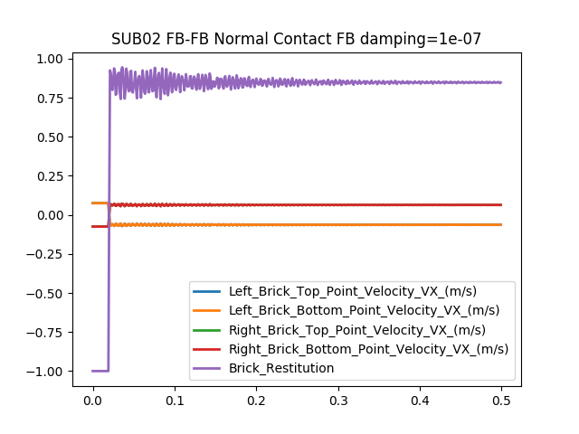
Fig. 79 Example 81array: example figure generated by post–processing 81fbi.py results.

In this example the modal base is generate “on the fly”, hence you can simply run

solfec examples/81array/81fbi.py -form MODAL -fbmod 16

and then again to post–process. The reduced order impact test by default employs the same bases as the 81array.inp input deck. If you run

solfec examples/81array/81fbi.py -form RO

it will “tell”

Reading out/81fbi_RO_FB24_s1.0e-04_d1.0e-07_r0/FB1_base.pickle.gz failed --> you can run -form BC -genbase to genrate this file
Now trying to use examples/81array/81array_FB1_base.pickle.gz instead ...

When generating bases, e.g.

solfec examples/81array/81fbi.py -genbase -fbmod 72

bear in mind that the number of available modes will be less than that for the 81 array input decks – the displacement time history is “algebraically poorer” for the impact test. This will be signalled as follows

FB1: calculating 72 POD modes from 506 input vectors of size 432 ...
POD generation has failed --> it is possible that you tried to extract too many modes
                              try using [-fbmod a_smaller_number] and re-run

You can then reuse the existing results and just keep trying, e.g.

solfec examples/81array/81fbi.py -genbase -fbmod 32

will work. You can than run the reduced order analysis

solfec examples/81array/81fbi.py -form RO -fbmod 32

and post–process it (re–run again) to find out the restitution coefficient.

*

AGR stands for an Advanced Gass-cooled Reactor.

1

Ahmed, Khalid and Stojko, Stefan, “The non–linear seismic response of AGR core graphite brick slices – correlation of experimental and analytical results”, Earthquake Engineering & Structural Dynamics (1987), 159–188.

2

Ahmed, K. M., “The dynamic response of multi-layers AGR core brick arrays”, Nuclear Engineering and Design (1987), 1–66.