Pipe impact

This example, also included in TR1, illustrates the reduced order modeling functionality on a pipe impact problem. The input files for this example are located in the solfec-1.0/examples/reduced–order1 directory. These are:

• README – a text based specification of the problem

• ro1–fem–bc.py – finite element body co–rotated model

• ro1–fem–tl.py – finite element Total Lagrangian model

• ro1–reduced.py – finite element reduced order model

• ro1–lib.py – library functions used by other input files

• ro1–modred.py – calculation of a reduced POD base

• ro1–postp.py – post–processing script

• ro1–run–all.py – input file that runs all tests and generates all plots

• ro1–view.py – input file suitable for use with Solfec-1.0 viewer

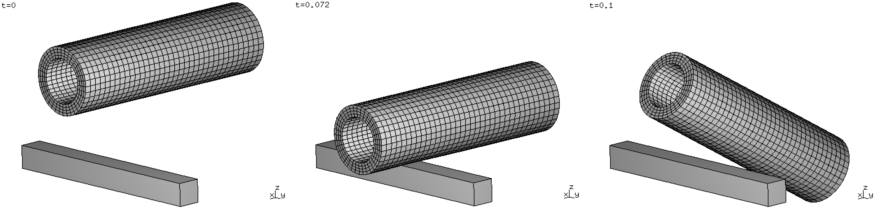
Fig. 65 Example reduced-order1: initial, impact, and final configurations (left to right).

An elastic pipe free falls onto a block obstacle. Fig. 65 illustrates the initial, impact and final configurations. The inner pipe radius is 0.01 m, its thickness is 0.005 m, and its length is 0.1 m. The pipe lowest point is initially located 0.025 m above the top surface of the block. Fig. 66 shows the characteristic points, used to extract results. Point p0 impacts the geometrical center of the block. Points p0, p1, p2, p3 are 0.025 m away from p4, when measuring along the pipe length. The pipe is made of \(36\times36\times4\) fully integrated trilinear hexahedral elements. The elastic properties of the pipe are \(E=1\mbox{E7 Pa}\), \(\nu=0.25\) and its density is \(\rho=1\mbox{E3 kg /}\mbox{m}^{3}\). The obstacle has dimensions \(0.01\times0.1\times0.01\mbox{ m}\) and it is modeled as a geometrical boundary which does not contribute mass. The gravity along the z–direction is \(-10\text{ m/s}^{2}\). The simulation time step is 0.001 s, the duration is 0.1 s, and the amount of damping is \(\eta=1\text{E-4}\). Schemes TL, BC, and BC–RO are compared. 100 co–rotated displacement samples from the Total Lagrangian solution and 6 rigid motion modes are used as input for the Python modred package, to produce 18 Proper Orthogonal Decomposition modes for the BC–RO approach.

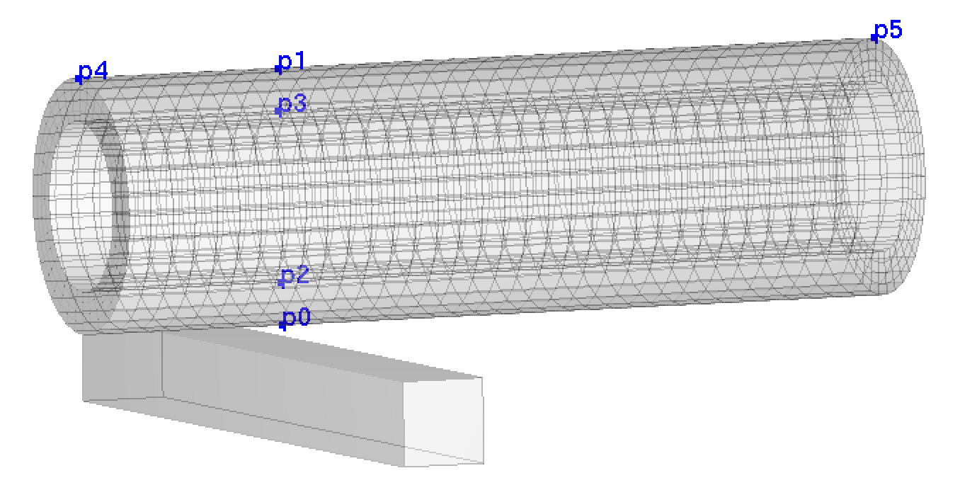
Fig. 66 Example reduced-order1: mesh characteristic points.

Fig. 67 illustrates the energy balance: in all cases the graphs coincide relatively well. While the BC approach closely follows the Total Lagrangian approach (TL), the reduced order BC–RO approach slightly deviates in its post-impact response. Similar general response characteristic can be seen in Fig. 68, Fig. 69, Fig. 70, where other types of results are compared: we have some variation in the post–impact response, while overall the results match. We note, that the rotation angle in Fig. 68 was calculated using

\[\text{angle}=\arcsin\left(\left|\frac{\text{p5}-\text{p4}}{\left|\text{p5}-\text{p4}\right|}\times\left(-1,0,0\right)\right|\right)\text{.}\]

Table 31 illustrates the runtime and storage statistics. The body co–rotational (BC) approach is about 6 times faster than TL; the reduced order (BC–RO) approach is about 50 time faster and requires about 50 times less storage. The animated output of this example can be seen in video 1.

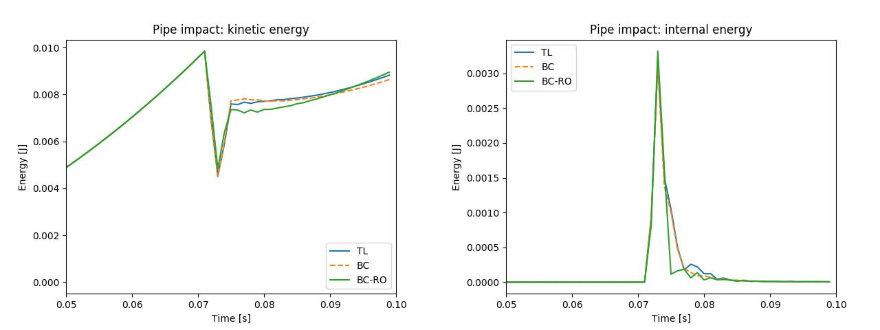
Fig. 67 Example reduced-order1: kinetic (left), and internal energy between \(t=0.05\text{s}\) and \(t=0.1\text{s}\).

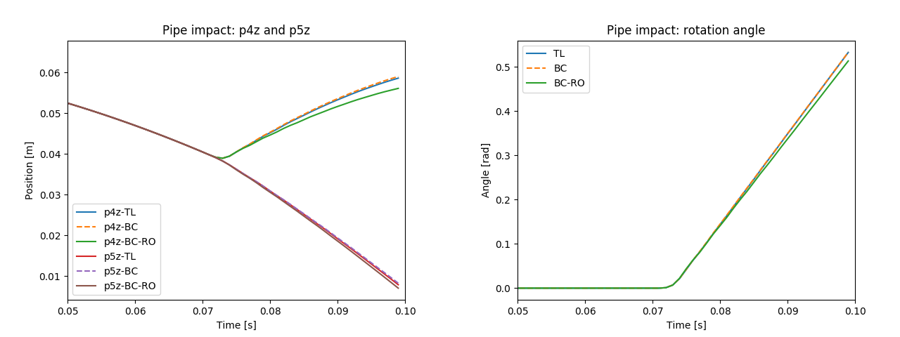
Fig. 68 Example reduced-order1: z–coordinates of points p4, p5 (left), and pipe rotation angle (about y) between \(t=0.05\text{s}\) and \(t=0.1\text{s}\).

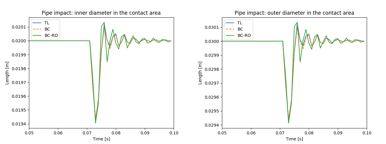
Fig. 69 Example reduced-order1: inner \(\left|\text{p2}-\text{p3}\right|\) (left), and outer \(\left|\text{p0}-\text{p1}\right|\) pipe diameter in the contact area between \(t=0.05\text{s}\) and \(t=0.1\text{s}\).

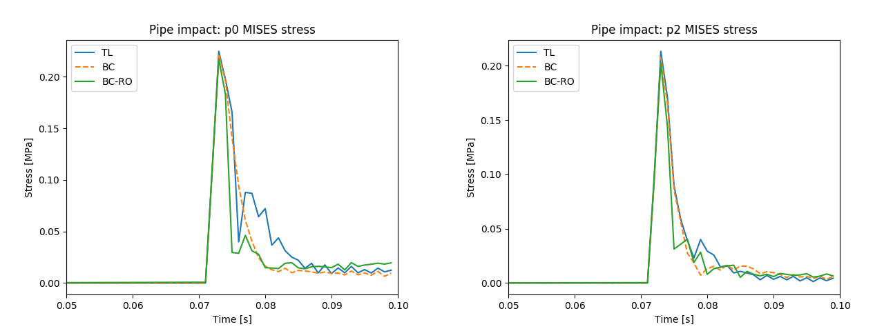
Fig. 70 Example reduced-order1: inner point p0 (left), and outer point p2 MISES stress between \(t=0.05\text{s}\) and \(t=0.1\text{s}\).

Table 31 Example reduced-order1: runtime and storage comparison.

Formulation	TL	BC	BC–RO
Runtime [s]	101	16.2	2.0
Storage [MB]	13	13	0.264

1(1,2)

An animation of the reduced-order1 pipe impact example.

Listing 8 Listing of ro1–fem–tl.py

import os, sys
dirpath = os.path.dirname(os.path.realpath(__file__))
execfile (dirpath + '/ro1-lib.py') # import library

# set up simulation
(sol, bod, stop) = ro1_simulation ('fem-tl')

# collect displacement samples
if sol.mode == 'WRITE' and not VIEWER():
  dsp = COROTATED_DISPLACEMENTS (sol, bod)
  rig = RIGID_DISPLACEMENTS (bod)

# run simulation and save displacemement samples
if sol.mode == 'WRITE':
  import time
  t0 = time.time()
  RUN (sol, NEWTON_SOLVER(), stop)
  t1 = time.time()
  print '\bFEM-TL runtime: %.3f seconds' % (t1-t0)
  if not VIEWER():
    print 'Saving displacement snapshots ...'
    import pickle
    pickle.dump(dsp, open('out/reduced-order1/dsp.pickle', 'wb')) 
    pickle.dump(rig, open('out/reduced-order1/rig.pickle', 'wb')) 

# read and save time histories
if sol.mode == 'READ' and not VIEWER():
  ro1_read_histories (sol, bod, 'fem-tl')

Listing 8 exemplifies the Total Lagrangian analysis input file. The simulation creation code is hidden inside of the library subroutine ro1_simulation, which returns the SOLFEC object, the pipe BODY object and the duration of the analysis, stop, in line 6. When Solfec-1.0 is opened in 'WIRITE' mode (no results exist) and without the graphical viewer (–v switch not used), we sample co–rotated deformable and rigid displacements in lines 10 and 11. COROTATED_DISPLACEMENTS and RIGID_DISPLACEMENTS commands are respectively used. Further, the simulation is run and the sampled displacements saved in lines 14–24. In case Solfec-1.0 is opened in 'READ' mode, in line 28, existing results are processed and time histories are extracted using a library routine ro1_read_histories. For comparison Listing 9 includes the BC–RO analysis input code. Since most of the input code is inside ro1–lib.py this file is even shorter. The sampled displacements are used by ro1–modred.py, invoked internally from within ro1_simulation, when creating the reduced order model of the pipe body. This is depicted in lines 34–49 of Listing 10.

Listing 9 Listing of ro1–reduced.py

import os, sys
dirpath = os.path.dirname(os.path.realpath(__file__))
execfile (dirpath + '/ro1-lib.py') # import library

# set up simulation
(sol, bod, stop) = ro1_simulation ('reduced')

# run simulation
if sol.mode == 'WRITE':
  import time
  t0 = time.time()
  RUN (sol, NEWTON_SOLVER(), stop)
  t1 = time.time()
  print '\bBC-RO runtime: %.3f seconds' % (t1-t0)

# read and save time histories
if sol.mode == 'READ' and not VIEWER():
  ro1_read_histories (sol, bod, 'reduced')

Listing 10 Listing of a portion of ro1–lib.py responsible for creation of the pipe body.

  if path_string == 'fem-tl':
    bod = BODY (sol, 'FINITE_ELEMENT', msh, mat, form = 'TL')
  elif path_string == 'fem-bc':
    bod = BODY (sol, 'FINITE_ELEMENT', msh, mat, form = 'BC')
  else:
    try:
      import pickle
      podbase = pickle.load(open('out/reduced-order1/podbase.pickle', 'rb'))
    except:
      print 'File out/reduced-order1/podbase.pickle not found',
      print '--> running ro0-modred.py ...'
      execfile (dirpath + '/ro1-modred.py')
      try:
	import pickle
	podbase = pickle.load(open('out/reduced-order1/podbase.pickle', 'rb'))
      except:
        print 'Running ro0-modred.py has failed --> report a bug!' 
	import sys
	sys.exit(0)
    bod = BODY (sol, 'FINITE_ELEMENT', msh, mat, form = 'BC-RO', base = podbase)

To run this example and generate figures presented here, enter Solfec-1.0 source directory and type

solfec examples/reduced-order1/ro1-run-all.py

After all progress messages cease, figures are saved as out/reduced-order1/*.png files. To interactively view the animated bar, as in video 1, call

solfec -v examples/reduced-order1/ro1-view.py

You can type o in order to highlight the output path in the viewer and see which model you are currently looking at. You can switch between models using < and >. Right–click the mouse button to activate a drop–down menu and see other available options and keyboard shortcuts.