Rotating bar

This is a simplest application of the reduced order modeling functionality. This example is also included in TR1: having a look into this technical report may be helpful. The input files for this example are located in the solfec-1.0/examples/reduced–order0 directory. These are:

• README – a text based specification of the problem

• ro0–convtest.py – convergence test runs and plotting

• ro0–elong.py – elongation test runs and time history plotting

• ro0–energy.py – energy balance test runs and time history plotting

• ro0–gen–bases.py – calculation of a reduced POD base

• ro0–lib.py – library functions used by other input files

• ro0–run–all.py – input file that runs all tests and generates all plots

• ro0–view.py – input file suitable for use with Solfec-1.0 viewer

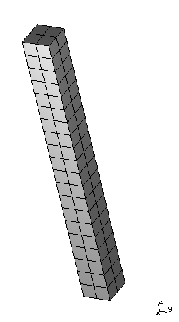
Fig. 60 Example reduced-order0: geometry of the \(2\times2\times20\) mesh.

A prismatic bar with \(x,y,z\) dimensions \(0.1\times0.1\times1\mbox{ m}\) and material parameters \(E\in\left\{ 200\mbox{E4 Pa},200\mbox{E9 Pa}\right\}\), \(\nu=0.26,\rho=7.8\mbox{E3 kg /}\mbox{m}^{3}\) is rotating about the \(x\)–axis with an initial angular velocity of \(1\mbox{ rad/s}\). We use the smaller Young’s modulus in most demonstrations since in this case the time scales of the rigid and deformable motions are not far apart. For \(E=200\mbox{E9 Pa}\) the material parameters correspond to steel. In this case the time scale of elastic deformations is much faster then that of the rigid rotation. We use this material to test performance of the proposed integrators when applied with large time steps. In what follows, unless stated otherwise, the value \(E=200\mbox{E4}\) is used by default.

1(1,2)

An animation of the reduced-order0 rotating bar example.

The bar is discretized with \(2\times2\times20\) fully integrated trilinear hexahedral elements, Fig. 60 and animation 1. This results in 576 degrees of freedom for the full order model. For the reduced order BC–RO approach we used 100 co–rotated displacement samples from the Total Lagrangian solution (with rigid rotation factored out) and 6 rigid motion modes (generated algebraically) as input for the Python modred package and calculated 11 Proper Orthogonal Decomposition modes. In the current example, we also include the BC–MODAL approach, for which the 6 rigid modes where combined with deformable modes 14, 19, 26, 34, 39 (of the initial linearized system), picked by hand as visually corresponding to the predominantly longitudinal deformation of the bar. Hence, the BC–MODAL case also had 11 degrees of freedom.

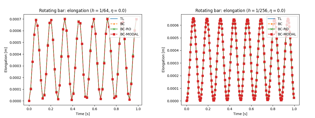
Fig. 61 Example reduced-order0: time history of the elongation for \(h\in\left\{ 1/64\mbox{s},1/256\mbox{s}\right\}\) and \(1\mbox{s}\) runs.

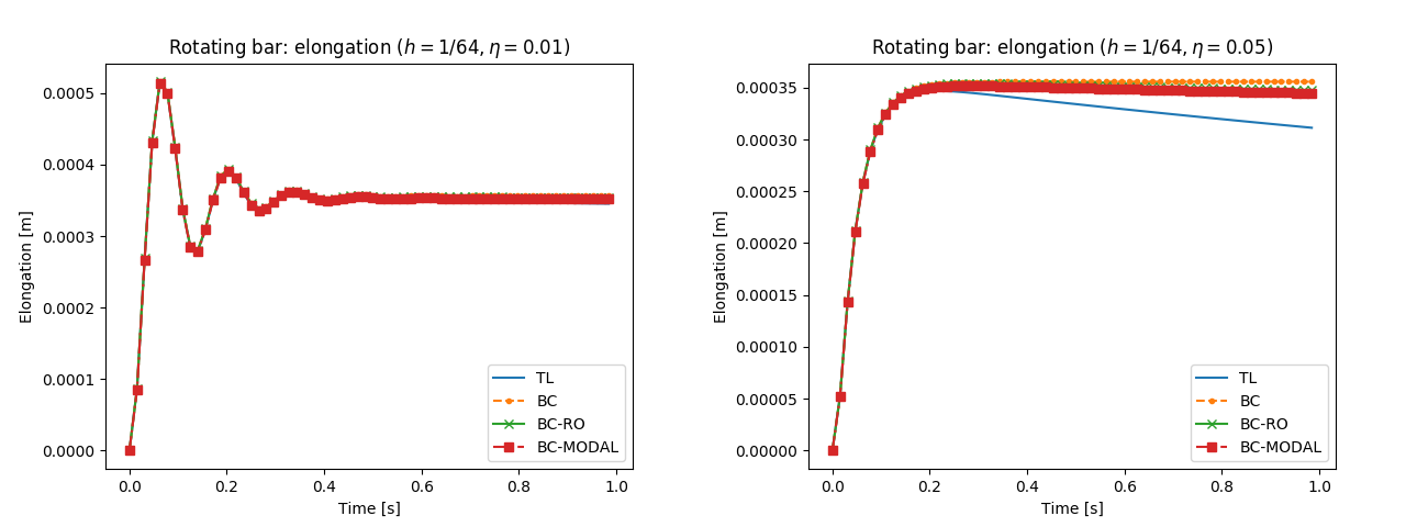
Fig. 62 Example reduced-order0: time history of the elongation for \(h=1/64\mbox{s}, \eta\in\left\{ 0.01,0.05\right\}\) and \(1\mbox{s}\) runs.

We first compare the solutions for damped and undamped cases. Fig. 61 illustrates the time history of the elongation of the bar, measured between the top and bottom center nodes, for undamped \(1\mbox{s}\) runs with time steps \(h\in\left\{ 1/64\mbox{s},1/256\mbox{s}\right\}\). It can be seen that the results compare well between the formulations proposed here and the Total Lagrangian approach integrated in an analogous manner. A damped case is illustrated in Fig. 62 for the large time step of \(h=1/64\mbox{s}\). Also in this case the agreement is good. The Total Lagrangian based solution deviates from the co–rotational solution since for the TL the stiffness matrix magnitude changes with configuration, which affects the stiffness proportional damping. We can conclude the 5 deformable modes used by the BC–RO and BC–MODAL approaches represent well the longitudinal oscillation accompanying the rotational motion of the bar.

Listing 6 Listing of a portion of ro0–elong.py responsible for creation of Fig. 61

  execfile (dirpath + '/ro0-gen-bases.py')
  import matplotlib.pyplot as plt
  ro0_path_extension ('-elong')
  print '================'
  print 'Elongation plots'
  print '================'
  # Plot bar elongation history for:
  # - all schemes
  # - steps 1/64s and 1/256s
  # - damping 0.0
  step_denom = [64, 256]
  for div in step_denom:
    print 'Solving for step 1/%d and damping 0.0 ...' % div
    print 'FEM-TL ...',
    sol = ro0_model (1.0/div, 0.0, 'TL', verbose='%\n',
		     overwrite=True, runduration=1.0)
    print '\bFEM-BC ...',
    sol = ro0_model (1.0/div, 0.0, 'BC', verbose='%\n',
		     overwrite=True, runduration=1.0)
    print '\bFEM-BC-RO ...',
    sol = ro0_model (1.0/div, 0.0, 'BC-RO', pod_base,
	verbose='%\n', overwrite=True, runduration=1.0)
    print '\bFEM-BC-MODAL ...',
    sol = ro0_model (1.0/div, 0.0, 'BC-MODAL', modal_base,
	    verbose='%\n', overwrite=True, runduration=1.0)

    # open in 'READ' mode and retrieve time histories
    times = ro0_times (ro0_model (1.0/div, 0.0, 'TL'))
    l_tl = ro0_elongation (ro0_model (1.0/div, 0.0, 'TL'))
    l_bc = ro0_elongation (ro0_model (1.0/div, 0.0, 'BC'))
    l_bc_ro = ro0_elongation (ro0_model (1.0/div, 0.0,
                                         'BC-RO', pod_base))
    l_bc_modal = ro0_elongation (ro0_model (1.0/div, 0.0,
                                    'BC-MODAL', modal_base))

    print '\bPlotting elongation history h=1/%d, eta=0.0 ...' % div
    plt.clf ()
    plt.title ('Rotating bar: elongation ($h = 1/%d, \eta = 0.0$)' % div)
    plt.plot (times, l_tl, label='TL')
    plt.plot (times, l_bc, label='BC', ls='--', marker='.')
    plt.plot (times, l_bc_ro, label='BC-RO', ls='-', marker='x')
    plt.plot (times, l_bc_modal, label='BC-MODAL', ls='-.', marker='s')
    plt.xlabel ('Time [s]')
    plt.ylabel ('Elongation [m]')
    plt.legend(loc = 'upper right')
    plt.gcf().subplots_adjust(left=0.15)
    plt.savefig ('out/reduced-order0/ro0_elongation_h%d_d0.png' % div)

Looking at the input code that helped to generate the above results, we can start with file ro0–elong.py. Listing 6 includes a portion of this file responsible for generating Fig. 61. In line 9 we execute the ro0–gen–bases.py file which generates reduced order and modal bases variables pod_base and modal_base, used in lines 40 and 42. We then use a library routine ro0_path_extension to include into the output directory path an extension specific to the elongation history tests. All library ro0_* subroutines are included in ro0–lib.py file, executed at the start, not shown here. In line 20 we start a loop over two time steps: 1/64s and 1/256s. For each time step, we run 1.0s long simulations using 'TL', 'BC', 'BC-RO, 'BC-MODAL' formulations, in lines 23–33, and then read the resulting time histories in lines 36–42. The ro0_model function creates a rotating bar model, runs the analysis, or reads the results, depending on parameters. The ro0_times function returners the time history of time itself. The ro0_elongation function reads and returns the time history of bar elongation, given a SOLFEC object in 'READ' mode as an input. Finally, in lines 44–55, we use matplotlib to generate figures that contribute to Fig. 61.

Listing 7 Listing of ro0–gen–bases.py

# import model library routines
import os
dirpath = os.path.dirname(os.path.realpath(__file__))
execfile (dirpath + '/ro0-lib.py')

# Initialise POD and modal bases
try:
  import pickle
  pod_base = pickle.load(open('out/reduced-order0/pod_base.pickle', 'rb'))
  modal_base = pickle.load(open('out/reduced-order0/modal_base.pickle', 'rb'))
except:
  ro0_path_extension ('-init')
  print '=============='
  print 'Initialization'
  print '=============='
  sol = ro0_model (1.0/256, 0.0, 'TL', verbose='%\n', overwrite=True)
  print 'Samping displacements ...',
  rig = RIGID_DISPLACEMENTS (sol.bodies[0])
  defo = COROTATED_DISPLACEMENTS (sol, sol.bodies[0])
  RUN (sol, NEWTON_SOLVER(), 1.0)
  print '\bCalculating POD base ...'
  pod_base = ro0_POD_base (rig, defo, verbose=True)
  print 'Calculating modal base ...'
  modal_base = ro0_modal_base ()

  # Save POD and modal bases
  import pickle
  pickle.dump(pod_base, open('out/reduced-order0/pod_base.pickle', 'wb')) 
  pickle.dump(modal_base, open('out/reduced-order0/modal_base.pickle', 'wb')) 

Listing 7 includes the ro0–gen–bases.py file. Because this code is used by multiple tests, in lines 9–10 we first attempt to read existing bases: one of the input files could have been called already and those bases may have been saved. If this is not the case, in lines 12–29 we generate and save the reduced order and modal bases. To generate the proper orthogonal decomposition reduced order base, we first create a Total Lagrangian model, in line 16, but do not run it yet (the runduration parameter of ro0_model is not used). Instead, we used the RIGID_DISPLACEMENTS and COROTATED_DISPLACEMENTS commands in order to sample rigid and co–rotated deformable displacements, and then run the analysis in line 20. The rigid displacements rig and the sampled deformable displacements defo are then passed to the library routine ro0_POD_base which employs the modred package to calculate the reduced base. Following this, in line 24, the modal base is generated using library call to ro0_modal_base, which employs Solfec-1.0’s utility function MODAL_ANALYSIS in order to calculate the modal base. Finally, the results are saved in lines 28 and 29.

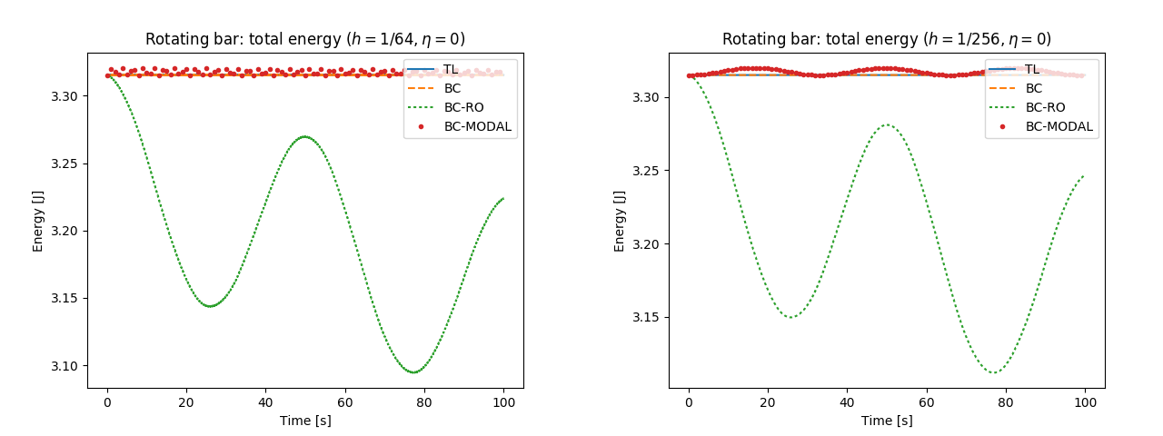
Fig. 63 Example reduced-order0: time history of total energy for \(h\in\left\{ 1/64\mbox{s},1/256\mbox{s}\right\}\) and \(100\mbox{s}\) runs.

Fig. 63 illustrates the time history of the total energy of the bar for 100s runs with time steps \(h\in\left\{ 1/64\mbox{s},1/256\mbox{s}\right\}\). For all but the BC–RO approach, the small oscillation of energy remains bounded with time. The full space co–rotational BC approach is better behaved than BC–MODAL: in nearly coincides with the Total Lagrangian approach. The relatively small oscillation of energy, present in TL, BC, and BC–MODAL cases, is characteristic for the adopted time stepping and it has been also demonstrated 2 on simpler model problems. The larger oscillation and dissipation of energy, clear in case of the BC–RO approach, remains a shortcoming and it may be addressed in future revisions of TR1. We note, that the ro0–energy.py input file was used to generate Fig. 63.

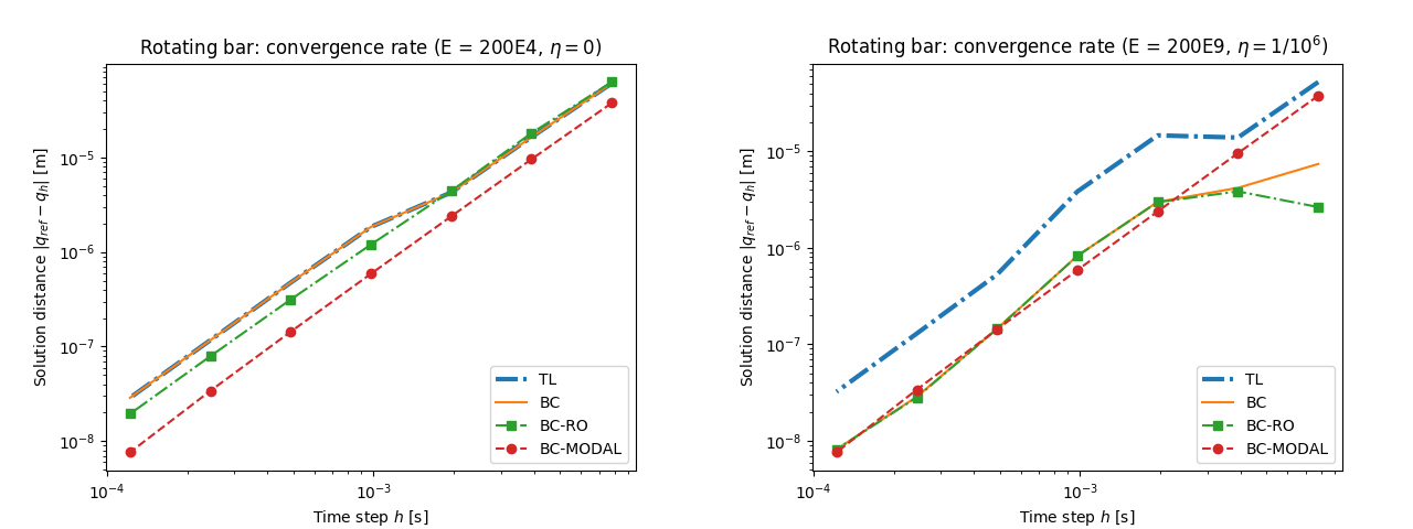
Fig. 64 Example reduced-order0: second order convergence of displacements for soft undamped (\(E=200\mbox{E4, }\eta=0\)) and stiff damped (\(E=200\mbox{E9, }\eta=1/10^{6}\)) materials.

The second order convergence rate is illustrated in Fig. 64. Two cases are considered: undamped motion of a soft bar \(E=200\mbox{E4}\) and damped motion of stiff bar \(E=200\mbox{E9}\). In both cases the reference solution \(q_{ref}\) was obtained at time \(t=1/2^{4}\mbox{s}\) with time step \(h=1/2^{16}\mbox{s}\). For the softer material the time scales of the rigid and deformable motion are not far apart and hence it is easier to observe the second order convergence for larger time steps. For the stiffer model we used damping \(\eta=1/10^{6}\) in order to damp out the high frequency oscillations that could not be well represented for the large time steps used here. Fig. 64 was generated using the ro0–convtest.py input file.

To run this example and generate figures presented here, enter Solfec-1.0 source directory and type

solfec examples/reduced-order0/ro0-run-all.py

After several minutes, when progress messages cease, figures are saved as out/reduced-order0/*.png files. To interactively view the animated bar, as in video 1, call

solfec -v examples/reduced-order0/ro0-view.py

You can type o in order to highlight the output path in the viewer and see which model you are currently looking at. You can switch between models using < and >. Right–click the mouse button to activate a drop–down menu and see other available options and keyboard shortcuts.

2

ANM, 25(2–3): 297–302, 1997.