1,2,3–dimensional cube array acceleration dwell

This is a family of 1,2 and 3–dismenional examples demonstrating applications of the HYBRID_SOLVER on an array of cubes subject to a constant amplitude and frequency acceleration since dwell signal. The input files for these examples are located in:

• solfec-1.0/examples/hybrid–solver1 for the 1–dimensional array.

• solfec-1.0/examples/hybrid–solver2 for the 2–dimensional array.

• solfec-1.0/examples/hybrid–solver3 for the 3–dimensional array.

We focus on the 2–dimensional example, leaving the 1– and 3–dimensional cases for self–study. The solfec-1.0/examples/hybrid–solver2 directory contains:

• README – a text based specification of the problem

• hs2–parmec.py – including the Parmec input code

• hs2–solfec.py – including the Solfec-1.0 input code

• hs2–parmec–only.py – including the Parmec-only version of the example

• hs2–solfec–only.py – including the Solfec-1.0-only version of the example

• hs2–state–1.pvsm – ParaView state for animation 1

• hs2–state–2.pvsm – ParaView state for animation 2

• hs2–state–3.pvsm – ParaView state for Fig. 55

• hs2–state–4.pvsm – ParaView state for Fig. 56

• hs2–state–5.pvsm – ParaView state for Fig. 57

• hs2–state–6.pvsm – ParaView state for Fig. 58

Fig. 53 states the problem and describes the hybrid model.

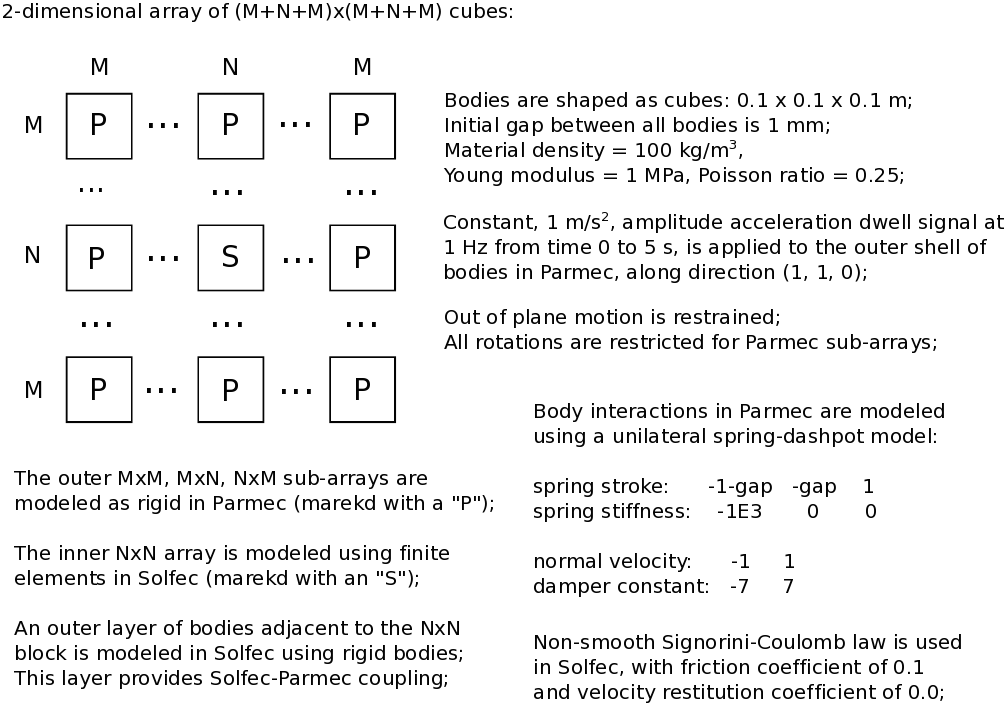
Fig. 53 Example hybrid-solver2: a 2–dimensional cube array acceleration dwell hybrid model

An actual array geometry is depicted in Fig. 54, where the color coding is as follows:

• blue – the outer Parmec bodies where acceleration sweep signal is applied

• yellow – the inner Parmec bodies interacting via spring–dashpot elements

• green – the boundary Parmec–Solfec-1.0 bodies, modeled in both codes

• grey – the inner Solfec-1.0 bodies, interacting via a non–smooth contact law

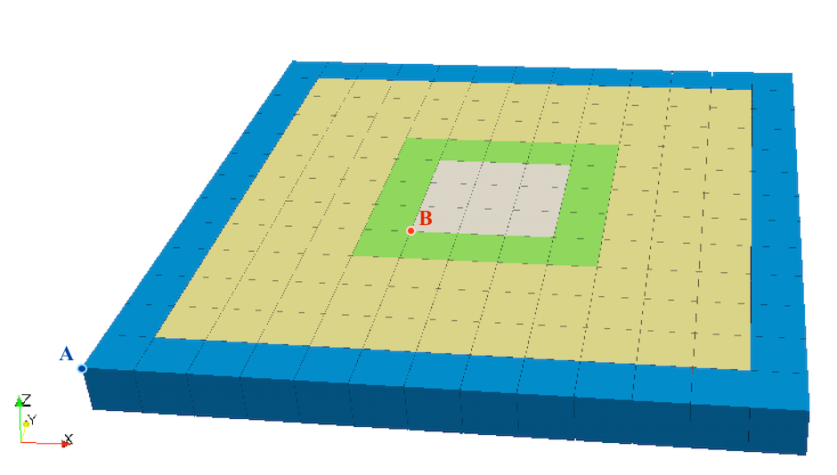
Fig. 54 Example hybrid-solver2: initial geometry.

Listing 4 includes the Parmec file hs2–parmec.py. Lines 1–8 define basic parameters of the model. We note, that it is possible to transform the current example into a sine sweep test by changing the “hifq” variable to a value greater than “lofq”. Also the size of the problem can be modified by altering the “N” and “M” parameters. Lines 10–25 are Python specific and help to find the path to the parmec source directory, in order to include the acceleration sweep generation script into the current system path. This is then used in line 30, and further until line 38, to set up the linear motion excitation vector, where the velocity time history, associated with the sine dwell signal, is used. Following definition of a translate cube creation function, in lines 43–58, the array of cubes is generated in lines 60–68. Then the prescribed motion is applied to the outer shell of cubes in lines 70–76. Finally, between the lines 78 and 98 contact spring–dashpot elements are defined and inserted into the model. For information, the critical time step estimation for the model is printed out in line 101.

Listing 4 Listing of hs2–parmec.py

# inherited from SOLFEC: M, N, gap, step, stop
lofq = 1 # low excitation frequency
hifq = 1 # high excitation freqency
amag = 1 # acceleration magnitude

# find path to parmec source directory in order
# to load the acceleration sweep signal script
import os, sys
def where(program):
  for path in os.environ["PATH"].split(os.pathsep):
    if os.path.exists(os.path.join(path, program)):
      return path
  return None
path = where('parmec4')
if path == None:
  print 'ERROR: parmec4 not found in PATH!'
  print '       Download and compile parmec;',
  print 'add parmec directory to PATH variable;'
  sys.exit(1)
print '(Found parmec4 at:', path + ')'
sys.path.append(os.path.join (path, 'python'))

# generate acceleration sweep signal;
# note that parmec will use the associated
# velocity signal, rather than the acceleration itself
from acc_sweep import *
(vt, vd, vv, va) = acc_sweep (step, stop, lofq, hifq, amag)
tsv = [None]*(len(vt)+len(vd))
tsv[::2] = vt
tsv[1::2] = vv
tsv = TSERIES (tsv) # velocity time series
ts0 = TSERIES (0.0) # constant, zero "time series"
linvel = (tsv, tsv, ts0) # linear motion excitation vector
angvel = (ts0, ts0, ts0) # angular motion excitation vector

# create material
matnum = MATERIAL (100, 1E6, 0.25)

# cube creation function
def cube (x, y):
  nodes = [x+0.0, y+0.0, 0.0,
	   x+0.1, y+0.0, 0.0,
	   x+0.1, y+0.1, 0.0,
	   x+0.0, y+0.1, 0.0,
	   x+0.0, y+0.0, 0.1,
	   x+0.1, y+0.0, 0.1,
	   x+0.1, y+0.1, 0.1,
	   x+0.0, y+0.1, 0.1]
  elements = [8, 0, 1, 2, 3, 4, 5, 6, 7, matnum]
  colors = [1, 4, 0, 1, 2, 3, 2, 4, 4, 5, 6, 7, 3]
  parnum = MESH (nodes, elements, matnum, colors)
  RESTRAIN (parnum, [0, 0, 1], [1, 0, 0, 0, 1, 0, 0, 0, 1])
  ANALYTICAL (particle=parnum)
  return parnum

# generate cube pattern
ijmap = {}
for i in range (0,M+N+M):
  for j in range (0,M+N+M):
    # skip the inner NxN Solfec block
    if i >= M and j >= M and i < M+N and j < M+N: continue
    else: # create the outer MxM, NxM, MxN blocks
      num = cube (i*(0.1+gap), j*(0.1+gap))
      ijmap[(i,j)] = num # map body numbers to (i,j)-grid

# prescribe sine dwell motion 
# of the outer-most shell of bodies
for (i,j) in ijmap:
  outer = [0, M+N+M-1]
  if i in outer or j in outer:
    num = ijmap[(i,j)]
    PRESCRIBE (num, linvel, angvel)

# spring-damper curves
spring_curve = [-1-gap, -1E3, -gap, 0, 1, 0]
damper_curve = [-1, -7, 1, 7]

# insert contact springs
ijmax = M+N+M-1
for (i, j) in ijmap:
  if i < ijmax and not (i == M-1 and j in range(M,M+N)):
    p1 = (i*(0.1+gap)+0.1, j*(0.1+gap)+0.05, 0.05)
    p2 = (i*(0.1+gap)+0.1+gap, j*(0.1+gap)+0.05, 0.05)
    n1 = ijmap[(i,j)]
    n2 = ijmap[(i+1,j)]
    SPRING (n1, p1, n2, p2, spring_curve,
            damper_curve, (1, 0, 0))
  if j < ijmax and not (j == M-1 and i in range(M,M+N)):
    p1 = (i*(0.1+gap)+0.05, j*(0.1+gap)+0.1, 0.05)
    p2 = (i*(0.1+gap)+0.05, j*(0.1+gap)+0.1+gap, 0.05)
    n1 = ijmap[(i,j)]
    n2 = ijmap[(i,j+1)]
    SPRING (n1, p1, n2, p2, spring_curve,
            damper_curve, (0, 1, 0))

# FYI, print out critical time step information 
print 'PARMEC estimated critical time step:', CRITICAL()

#DEM (stop, step, 0.01)

Listing 5 includes the Solfec-1.0 file hs2–solfec.py. Lines 1–5 define the global model parameters. Lines 7–24 set up the SOLFEC object, bulk and surface materials, and a unit cube template. Lines 26–56 contain code creating the array of Solfec-1.0 bodies as well as the mapping between the Parmec and the Solfec-1.0 body numbers. The double loop starting in line 30 of Listing 5 mimics the double loop starting in line 62 of Listing 4. This way, it is easy to recreate the exact sequence of creation of Parmec bodies within the Solfec-1.0 input file. Hence, it is easy to construct the parmec2solfec dictionary mapping of body numbers, on the fly, while creating the Solfec-1.0 model. The inner Solfec-1.0 bodies (grey in Fig. 54) are created in lines 33–45. This same range of i, j indices is skipped in the Parmec input file (line 65 in Listing 4). Here, finite element bodies are created, based on a 2x2x2 hexahedral mesh. The z–direction of the bodies is fixed to keep them in plane. The rigid “boundary” bodies for the Solfec-1.0–Parmec overlap interface are created in lines 50–53. We note, that when a Solfec-1.0 input file is run in parallel (using solfec-mpi) some of the bodies that are created in the loop may actually reside on other processor ranks. Hence we test this using the HERE command and accordingly create valid fragments of the parmec2solfec mapping on each MPI rank. Such fragmentary mappings are brought together during initialization of the HYBRID_SOLVER. In line 56 the Parmec body index is advanced, as this line corresponds to line 67 in Listing 4, where Parmec bodies are created. The rest of the file is similar to that already detailed in the description of Listing 3, in the context of the two body impact example.

Listing 5 Listing of hs2–solfec.py

M = 5 # outer layers
N = 3 # inner layers
gap = 0.001 # betweeb bodies
step = 5E-4 # time step
stop = 5 # duration

# create solfec object
sol = SOLFEC ('DYNAMIC', step, 'out/hybrid-solver2')

# bulk and surface materials
mat = BULK_MATERIAL (sol, model = 'KIRCHHOFF',
  young = 1E6, poisson = 0.25, density = 100)
SURFACE_MATERIAL (sol,
  model = 'SIGNORINI_COULOMB', friction = 0.1)

# template cube nodes
nodes = [0.0, 0.0, 0.0,
         0.1, 0.0, 0.0,
	 0.1, 0.1, 0.0,
	 0.0, 0.1, 0.0,
	 0.0, 0.0, 0.1,
	 0.1, 0.0, 0.1,
	 0.1, 0.1, 0.1,
	 0.0, 0.1, 0.1]

# create the array of cubes
iparmec = 0 # parmec indexing
parmec2solfec = {} # boundary bodies mapping
isolfec = [] # solfec indexing
for i in range (0,M+N+M):
  for j in range (0,M+N+M):
    if i >= M and j >= M and i < M+N and j < M+N:
      # inner Solfec bodies
      msh = HEX (nodes, 2, 2, 2, 0, [0, 1, 2, 3, 4, 5])
      TRANSLATE (msh, (i*(0.1+gap), j*(0.1+gap), 0))
      p1 = msh.node(0)
      p2 = msh.node(2)
      p3 = msh.node(8)
      bod = BODY (sol, 'FINITE_ELEMENT', msh, mat)
      bod.scheme = 'DEF_LIM' # semi-implicit time integration
      bod.damping = 1E-4 # damping out free vibrations
      isolfec.append(bod.id)
      FIX_DIRECTION (bod, p1, (0, 0, 1))
      FIX_DIRECTION (bod, p2, (0, 0, 1))
      FIX_DIRECTION (bod, p3, (0, 0, 1))
    else:
      if (i in [M-1,M+N] and j in range(M,M+N)) or \
	 (j in [M-1,M+N] and i in range(M,M+N)) or \
	 (i in [M-1,M+N] and j in [M-1,M+N]):
	# Solfec-Parmec boundary
	msh = HEX (nodes, 1, 1, 1, 0, [0, 1, 2, 3, 4, 5])
	TRANSLATE (msh, (i*(0.1+gap), j*(0.1+gap), 0))
	p1 = msh.node(0)
	p2 = msh.node(1)
	p3 = msh.node(3)
	bod = BODY (sol, 'RIGID', msh, mat)
	FIX_DIRECTION (bod, p1, (0, 0, 1))
	FIX_DIRECTION (bod, p2, (0, 0, 1))
	FIX_DIRECTION (bod, p3, (0, 0, 1))
        # in parallel bod.id can be None for remote bodies, so
	if HERE(sol,bod):
	  bod.disable_rotation = 'ON'
	  parmec2solfec[iparmec] = bod.id
      iparmec = iparmec + 1 # next parmec body

# create Newton solver
ns = NEWTON_SOLVER ()

# parmec's output files are written to the same
# location as the input path; for that to be the solfec's
# output directory, we copy parmec's input file there
from shutil import copyfile
copyfile('examples/hybrid-solver2/hs2-parmec.py',
         'out/hybrid-solver2/hs2-parmec.py')


# create hybrid solver
hs = HYBRID_SOLVER ('out/hybrid-solver2/hs2-parmec.py',
                    1E-4, parmec2solfec, ns)

# set PARMEC output interval
hs.parmec_interval = 0.03;

import solfec as solfec # this is needed since 'OUTPUT' in Solfec
solfec.OUTPUT (sol, 0.03) # collides with 'OUTPUT' in Parmec

# run simulation
import time
start_time = time.time()
RUN (sol, hs, stop)
if RANK() == 0: print("--- %s seconds ---" % (time.time() - start_time))

# XDMF export
if sol.mode == 'READ' and not VIEWER():
  XDMF_EXPORT (sol, (0.0, stop),
    'out/hybrid-solver2/hs2-solfec', isolfec)

The example is run by invoking

solfec examples/hybrid-solfec2/hs2-solfec.py

which needs to be followed by a repeated call

solfec examples/hybrid-solfec2/hs2-solfec.py

in order to produce the XDMF–exported Solfec-1.0 results. These will be located in the ‘out/hybrid–solver2/hs2–solfec’ directory, relative to the solfec source directory, from where this example is conveniently called. The Parmec output files are located in the ‘out/hybrid–solver2’ directory. While Solfec-1.0 viewer can be used to view and post–process the Solfec-1.0 part of the results without depending on the exported XDMF files, ParaView can be used to post–process the generated .xmf files. The application of ParaView can be simplified by utilising the two state .pvsm files distributed with the example: by selecting “File/Load State…” menu choice in ParaView one can load a pre–set post–processing state. The videos included below depict the forced motion of the hybrid system, visualised using the two enclosed states files.

1

ParaView animation based on the state file hs2–state–1.pvsm.

2

ParaView animation based on the state file hs2–state–2.pvsm.

Fig. 55 and Fig. 56 respectively show the linear velocity magnitude time history and the displacement magnitude time history, at points A (Parmec) and B (Solfec-1.0), marked out in Fig. 54. These plots were generated using ParaView’s “Plot Selection Over Time” feature.

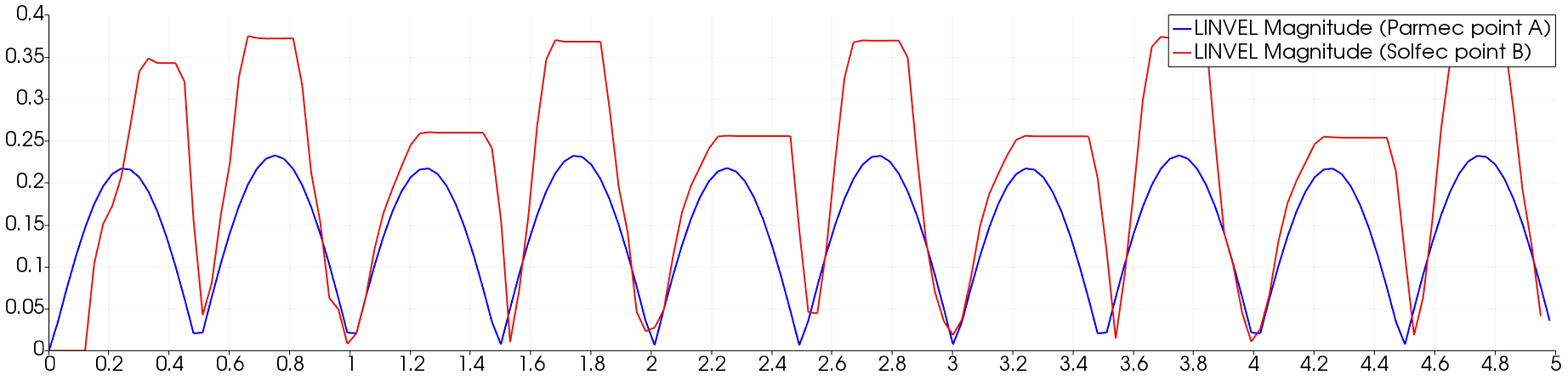
Fig. 55 Example hybrid-solver2: Linear velocity magnitude history at points A and B (Fig. 54).

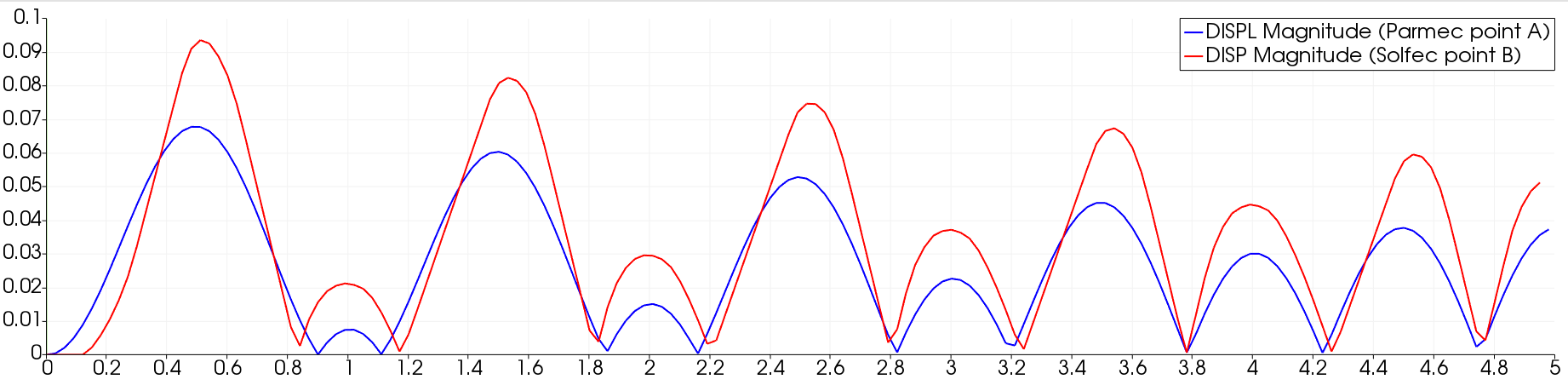
Fig. 56 Example hybrid-solver2: Displacement magnitude history at points A and B (Fig. 54).

Our current presentation is oriented at demonstrating the capability and performance aspects of the proposed framework. Therefore we did not attempt to consistently model a uniform physical system by means of the three approaches: Solfec-1.0-only, Parmec-only and hybrid. The physical parameters of the finite element (FE) Solfec-1.0-only model do not match those of the simplified Parmec-only model: the FE model is stiffer then the mass-and-spring model. The hybrid model thus represents a stiff inclusion surrounded by a softer surrounding material, rather than a uniform material modeled by means of two approaches. We did not attempt to fine-tune the physical parameters of the three models, apart from choosing parameters that resulted in stable simulations at a practical time step size. Below, in Fig. 57 and Fig. 58, we include comparisons of linear velocity magnitude and displacement magnitude, between the three approaches, recorded at point B of the geometry depicted in Fig. 54. It is quite clear that finite element based Solfec-1.0-only model has quite different dynamic response when compared with the latter two approaches. The Parmec-only and hybrid approaches have similar responses because the softer surrounding material dominates the hybrid model and determines the motion of the stiffer inclusion.

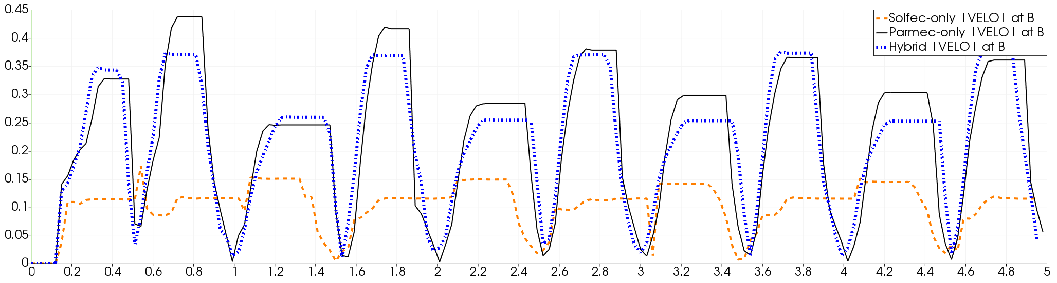
Fig. 57 Example hybrid-solver2: Velocity magnitude time history, at point B, for the three modeling approaches.

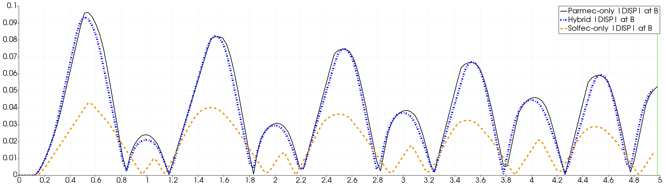
Fig. 58 Example hybrid-solver2: Displacement magnitude time history, at point B, for the three modeling approaches.

Finally, the most basic comparison of the practical advantage of simplified modeling is depicted in Table 27. The Solfec-1.0-only approach takes about 18 minutes to complete calculations. The most simplified Parmec-only approach takes only 10 seconds and is 105 times faster. The hybrid approach, on the other hard, which includes both rigid bodies (modeled in Parmec) and finite element bodies (modeled in Solfec-1.0) takes about 5 minutes to complete. This is 3.4 times faster than the Solfec-1.0-only case, and 31 times slower than Parmec-only. All Solfec-1.0 calculations were done using 4 MPI processes, while Parmec calculations took full advantage of a 4-core 2.3 GHz Intel Core i7 CPU on a MacBook Pro laptop (mid 2012 model).

Table 27 2D array runtime comparison, between the NSCD (Solfec-1.0), DEM (Parmec) and hybrid approaches.

Approach	Solfec-1.0-only					Parmec-only	Hybrid
Runtime [sec]	1053					10	308