A two–body impact problem
This is a simplest application of the HYBRID_SOLVER. The input files for this example are located in the solfec-1.0/examples/hybrid–solver0 directory. These are:
README – a text based specification of the problem
hs0–parmec.py – including the Parmec input code
hs0–solfec–1.py – including the simpler version of the Solfec-1.0 input code
hs0–solfec–2.py – Solfec-1.0 input file demonstrating a more elaborate usage of Parmec and Solfec-1.0 features
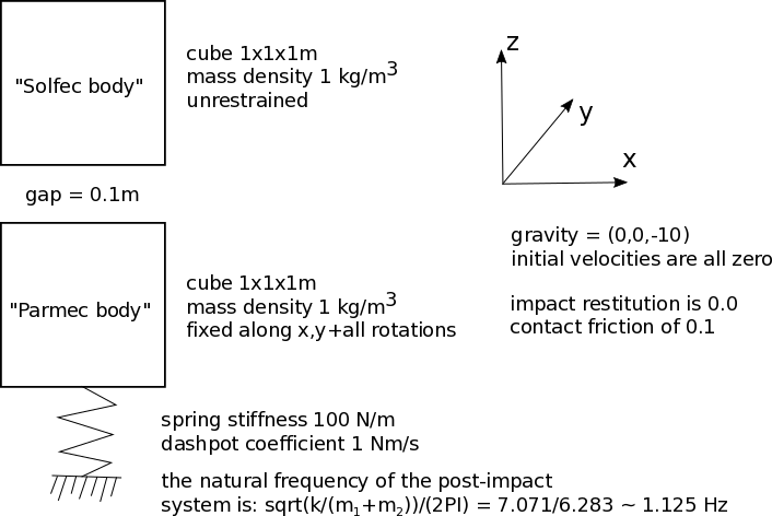
Fig. 50 Example hybrid-solver0: a two body impact problem
Fig. 50 states the problem. Both, the upper “Solfec-1.0” body and the lower “Parmec” body are modeled as rigid. The upper body falls under gravity and hits the lower body, initiating vibrations. There is no impact restitution between the two bodies, hence the two bodies stay and vibrate together, following the initial impact. We use this simple example to illustrate the methodology of creating a hybrid model.
Listing 1 includes the Parmec file hs0–parmec.py. The material is created in line 1 and the meshed lower cube is created in line 16. The cube’s motion is restrained along x, y translations and x, y, z rotations in line 18. The elastic spring is created in line 20. We note, that no damping is applied and that the spring direction is fixed along z. Gravity is applied in line 23. This concludes the input file.
 1matnum = MATERIAL (1, 1, 0.25)
 2
 3nodes = [0, 0, 0,
 4         1, 0, 0,
 5	 1, 1, 0,
 6	 0, 1, 0,
 7	 0, 0, 1,
 8	 1, 0, 1,
 9	 1, 1, 1,
10	 0, 1, 1]
11
12elements = [8, 0, 1, 2, 3, 4, 5, 6, 7, matnum]
13
14color = 1
15
16parnum = MESH (nodes, elements, matnum, color)
17
18RESTRAIN (parnum, [1, 0, 0, 0, 1, 0], [1, 0, 0, 0, 1, 0, 0, 0, 1])
19
20SPRING (parnum, (0.5, 0.5, 0.0), -1, (0.5, 0.5, -1.0),
21        spring = [-1, -100, 1, 100], direction = (0, 0, 1))
22
23GRAVITY (0.0, 0.0, -10.0)
24
25#DEM (10, 0.01)
The “DEM” command in line 25 can be uncommented to run parmec standalone and test this example:
parmec4 examples/hybrid-solver0/hs0-parmec.py
This is useful at a stage of creating and testing of an input file: the output files generated into the hybrid–solver0 directory and be viewed using ParaView.
Note
For the sake of using hs0–parmec.py as Parmec input in Solfec-1.0’s HYBRID_SOLVER, the “DEM” command in line 25 should remain commented out.
Listing 2 includes the Solfec-1.0 file hs0–solfec–1.py. SOLFEC object is created in line 3, specifying the output directory as ‘out/hybrid–solver0’ (relative where solfec is run from). Gravity is applied in line 5. Volumetric “bulk” material is created in line 7 and “suraface material” for contact interactions is created in line 10. Then the lower body “bod1” is created in line 22. This is a boundary body, coinciding with the Parmec body defined in line 16 of Listing 1. This body will be used to transfer forces between Solfec-1.0 and Parmec, and its motion will be driven by the Parmec model. The upper body “bod2” is created in line 26. In both cases Solfec-1.0’s MESH object is used to define geometry.
 1step = 0.01
 2
 3sol = SOLFEC ('DYNAMIC', step, 'out/hybrid-solver0')
 4
 5GRAVITY (sol, (0, 0, -10))
 6
 7mat = BULK_MATERIAL (sol, model = 'KIRCHHOFF',
 8       young = 1, poisson = 0.25, density = 1)
 9
10SURFACE_MATERIAL (sol, model = 'SIGNORINI_COULOMB', friction = 0.1)
11
12nodes = [0, 0, 0,
13         1, 0, 0,
14	 1, 1, 0,
15	 0, 1, 0,
16	 0, 0, 1,
17	 1, 0, 1,
18	 1, 1, 1,
19	 0, 1, 1]
20
21msh = HEX (nodes, 1, 1, 1, 0, [0, 1, 2, 3, 4, 5])
22bod1 = BODY (sol, 'RIGID', msh, mat) # boundary bodies are rigid
23
24FIX_DIRECTION (bod1, tuple(nodes[0:3]), (1, 0, 0))
25FIX_DIRECTION (bod1, tuple(nodes[0:3]), (0, 1, 0))
26FIX_DIRECTION (bod1, tuple(nodes[3:6]), (1, 0, 0))
27FIX_DIRECTION (bod1, tuple(nodes[12:15]), (1, 0, 0))
28FIX_DIRECTION (bod1, tuple(nodes[12:15]), (0, 1, 0))
29FIX_DIRECTION (bod1, tuple(nodes[15:18]), (1, 0, 0))
30
31msh = HEX (nodes, 2, 2, 2, 0, [0, 1, 2, 3, 4, 5])
32TRANSLATE (msh, (0, 0, 1.1))
33bod2 = BODY (sol, 'RIGID', msh, mat)
34
35ns = NEWTON_SOLVER ()
36
37# nubering of bodies in Parmec starts from 0 hence below we
38# use dictionary {0 : bod1.id} as the parmec2solfec mapping
39hs = HYBRID_SOLVER ('examples/hybrid-solver0/hs0-parmec.py',
40                    step, {0 : bod1.id}, ns)
41
42import solfec as solfec # this is needed since 'OUTPUT' in Solfec
43solfec.OUTPUT (sol, 0.03) # collides with 'OUTPUT' in Parmec
44
45RUN (sol, hs, 10)
The Newton solver is created next in line 28. It will be used internally by the hybrid solver in order to resolve (non–smooth) contact interactions between the two bodies. The HYBRID_SOLVER itself is created further, in line 32. We pass the full relative path to the parmec input file ‘examples/hybrid-solver0/hs0-parmec.py’, which implies that the example will be run from the solfec source directory. The Solfec-1.0 time step is used as the upper bound for the Parmec step. Knowing that Parmec numbers bodies starting from zero, we create a simple dictionary mapping, {0 : bod1.id}, to define the “boundary bodies” through which forces are passed between the two codes. Finally, we pass the Newton solver object “ns” as the last argument.
We note, that Parmec output intervals are not specified in this invocation of the hybrid solver. This means that Parmec will not create output files during the simulation. In lines 35 and 36 we define the Solfec-1.0 output interval. Because the “OUTPUT” commands coincide in both codes, we need to explicitly call the Solfec-1.0 command in this case. The input file is concluded with the “RUN” command (line 38), which executes a 10 second long simulation of the hybrid model.
The example is run by calling
solfec examples/hybrid-solver0/hs0-solfec-1.py
from within the solfec source directory. After calculations are finished, this can be followed by viewing the animated results by invoking
solfec -v examples/hybrid-solver0/hs0-solfec-1.py
An example animation is included below:
Listing 3 includes the second Solfec-1.0 file hs0–solfec–2.py. This input file demonstrates several more elaborate features of the HYBRID_SOLVER and of Solfec-1.0 input usage in general:
creation of Parmec output files (lines 32–36)
creation of Parmec time histories (lines 38–40)
runtime plotting from Solfec-1.0 (lines 42–51)
an application of matplotlib within Solfec-1.0 input file (lines 59–73)
XDMF export of Solfec-1.0 results (lines 75–80)
 1# as in hs0-solfec-1.py
 2step = 0.01
 3sol = SOLFEC ('DYNAMIC', step, 'out/hybrid-solver0')
 4GRAVITY (sol, (0, 0, -10))
 5mat = BULK_MATERIAL (sol, model = 'KIRCHHOFF',
 6      young = 1, poisson = 0.25, density = 1)
 7SURFACE_MATERIAL (sol, model = 'SIGNORINI_COULOMB', friction = 0.1)
 8nodes = [0, 0, 0, 1, 0, 0, 1, 1, 0, 0, 1, 0,
 9         0, 0, 1, 1, 0, 1, 1, 1, 1, 0, 1, 1]
10msh = HEX (nodes, 1, 1, 1, 0, [0, 1, 2, 3, 4, 5])
11bod1 = BODY (sol, 'RIGID', msh, mat) # boundary bodies are rigid
12FIX_DIRECTION (bod1, tuple(nodes[0:3]), (1, 0, 0))
13FIX_DIRECTION (bod1, tuple(nodes[0:3]), (0, 1, 0))
14FIX_DIRECTION (bod1, tuple(nodes[3:6]), (1, 0, 0))
15FIX_DIRECTION (bod1, tuple(nodes[12:15]), (1, 0, 0))
16FIX_DIRECTION (bod1, tuple(nodes[12:15]), (0, 1, 0))
17FIX_DIRECTION (bod1, tuple(nodes[15:18]), (1, 0, 0))
18msh = HEX (nodes, 2, 2, 2, 0, [0, 1, 2, 3, 4, 5])
19TRANSLATE (msh, (0, 0, 1.1))
20bod2 = BODY (sol, 'RIGID', msh, mat)
21ns = NEWTON_SOLVER ()
22
23# simulation end time
24stop = 10.0
25
26# parmec's output files are written to the same
27# location as the input path; for that to be the solfec's
28# output directory, we copy parmec's input file there
29from shutil import copyfile
30copyfile('examples/hybrid-solver0/hs0-parmec.py',
31         'out/hybrid-solver0/hs0-parmec.py')
32
33# nubering of bodies in Parmec starts from 0 hence below we
34# use dictionary {0 : bod1.id} as the parmec2solfec mapping
35hs = HYBRID_SOLVER ('out/hybrid-solver0/hs0-parmec.py',
36                    step, {0 : 1}, ns)
37
38# parmec module becomes available
39import parmec as parmec # after creation of the HYBRID_SOLVER
40tms0 = parmec.TSERIES ([0, 0.03, 5, 0.03, 5+step, 0.1, stop, 0.1])
41hs.parmec_interval = (tms0, 0.03) # variable output file interval
42                             #and constant output history interval
43
44# parmec time history plots are collected at runtime
45t_parmec = parmec.HISTORY ('TIME')
46dz_parmec = parmec.HISTORY ('DZ', 0)
47
48# solfec time history plots at runtime
49# can be collected via a callback
50t_solfec = []
51dz_solfec = []
52def plot_callback(sol, bod):
53  t_solfec.append(sol.time)
54  disp = DISPLACEMENT(bod, bod.center)
55  dz_solfec.append(disp[2])
56  return 1
57CALLBACK (sol, 0.03, (sol, bod2), plot_callback)
58
59import solfec as solfec # this is needed since 'OUTPUT' in Solfec
60solfec.OUTPUT (sol, 0.03) # collides with 'OUTPUT' in Parmec
61
62# run simulation
63RUN (sol, hs, stop)
64
65# plot time histories
66if sol.mode == 'WRITE' and not VIEWER():
67  try:
68    import matplotlib.pyplot as plt
69    print 'Plotting time histories...'
70    plt.clf ()
71    plt.plot (t_parmec, dz_parmec, label = 'lower body (parmec)')
72    plt.plot (t_solfec, dz_solfec, label = 'upper body (solfec)')
73    plt.legend (loc = 'upper right')
74    plt.xlim ((0, stop))
75    plt.xlabel ('time $(s)$')
76    plt.ylabel ('dz $(m)$')
77    plt.savefig ('out/hybrid-solver0/hs0-dz.png')
78  except:
79    print 'Plotting using matplotlib has failed.'
80
81# XDMF export
82if sol.mode == 'WRITE' and not VIEWER():
83  print 'Run one more times to export XDMF files!'
84elif sol.mode == 'READ' and not VIEWER():
85  XDMF_EXPORT (sol, (0.0, stop),
86    'out/hybrid-solver0/hs0-solfec', [bod2])
When the hybrid modeling is used, the Parmec library will generate output files if the Parmec output interval has been set. Enabling this feature is demonstrated in lines 32–36, where the “parmec_interval” parameter of the hybrid solver is set to value “(tms0, 0.03)”. The “tms0” object is Parmec’s TSERIES number, which in this case defines a variable output frequency for the Parmec output files. The second number, “0.03”, defines a constant time interval, at which Parmec time histories will be generated. These are requested in the following lines 38–40. This functionality (runtime generation of time histories) is matched in Solfec-1.0 via application of a callback function, as demonstrated in lines 42–51. These time histories are later used, in lines 59–73, in order to create a plot of the vertical displacement versus time, for the lower and the upper body. The result is seen in Fig. 51.
Note
Although there is no damping in the model, some dissipative behaviour is seen in Fig. 51. This is attributed to the force transfer mechanism between the two time–stepping methods, in Solfec-1.0 and Parmec. Constant forces from the previous time step in Parmec are used over the current time step in Solfec-1.0, and vice versa. The amount of this numerical dissipation decreases with time step size.
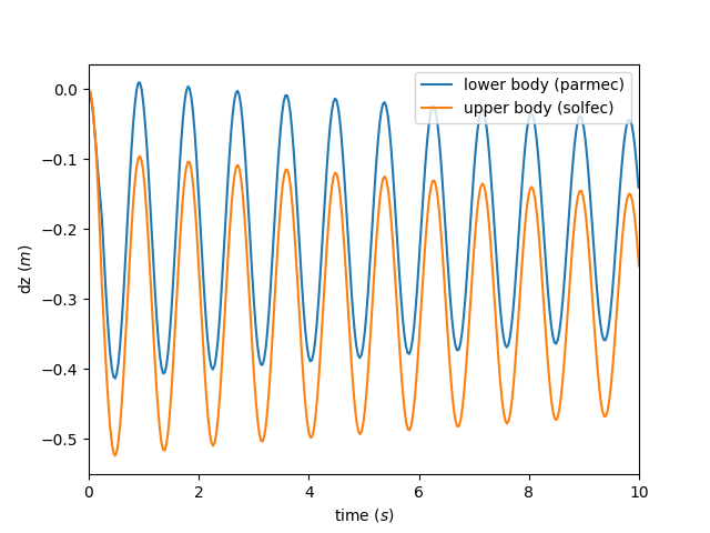
Fig. 51 Example hybrid-solver0: time histories of vertical displacement.
XDMF export is demonstrated in lines 75–80. We note, that Solfec-1.0 needs to be run for the second time, without the viewer -v parameter, in order for the actual export to occur:
solfec examples/hybrid-solver0/hs0-solfec-1.py
While Parmec output files, also in the XDMF format, are located in the ‘out/hybrid–solver0’ directory, the exported Solfec-1.0 XDMF files (.h5 and .xmf files) are placed inside of ‘out/hybrid–solver0/hs0–solfec’ directory. These files can be viewed using ParaView. An example session is depicted in Fig. 52.
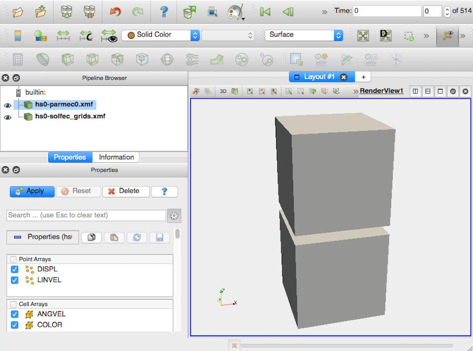
Fig. 52 Example hybrid-solver0: ParaView session exploiting the generated .xmf files.