Basics

We introduce basic notions here. Let us have a look at Fig. 3.

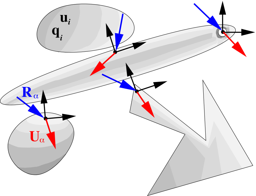
Fig. 3 A multi–body domain.

There are four bodies in the figure. Placement of each point of every body is determined by a configuration ${\mathbf{q}}_i$. Velocity of each point of every body is determined by a velocity ${\mathbf{u}}_i$. Let $\mathbf{q}$ and $\mathbf{u}$ collect configurations and velocities of all bodies. If the time history of velocity is known, the configuration time history can be computed as

(1)$$\mathbf{q}\left(t\right)=\mathbf{q}\left(0\right)+{\int }_0^t\mathbf{u}dt$$

The velocity is determined by integrating Newton’s law

(2)$$\mathbf{u}\left(t\right)=\mathbf{u}\left(0\right)+{\mathbf{M}}^{-1}{\int }_0^t(\mathbf{f}+{\mathbf{H}}^T\mathbf{R})dt$$

where $\mathbf{M}$ is an inertia operator (assumed constant here), $\mathbf{f}$ is an out of balance force, $\mathbf{H}$ is a linear operator, and $\mathbf{R}$ collects some point forces ${\mathbf{R}}_{\alpha }$. While integrating the motion of bodies, we keep track of a number of local coordinate systems (local frames). There are four of them in the above figure. Each local frame is related to a pair of points, usually belonging to two distinct bodies. An observer embedded at a local frame calculates the local relative velocity ${\mathbf{U}}_{\alpha }$ of one of the points, viewed from the perspective of the other point. Let $\mathbf{U}$ collect all local velocities. Then, we can find a linear transformation $\mathbf{H}$, such that

(3)$$\mathbf{U}=\mathbf{H}\mathbf{u}$$

In our case local frames correspond to constraints. We influence the local relative velocities by applying local forces ${\mathbf{R}}_{\alpha }$. This can be collectively described by an implicit relation

(4)$$\mathbf{C}(\mathbf{U},\mathbf{R})=\mathbf{0}$$

Hence, in order to integrate equations (1) and (2), at every instant of time we need to solve the implicit relation (4). Here is an example of a numerical approximation of such procedure

(5)$${\mathbf{q}}^{t+\frac{h}{2}}={\mathbf{q}}^t+\frac{h}{2}{\mathbf{u}}^t$$

(6)$${\mathbf{u}}^{t+h}={\mathbf{u}}^t+{\mathbf{M}}^{-1}h{\mathbf{f}}^{t+\frac{h}{2}}+{\mathbf{M}}^{-1}{\mathbf{H}}^T\mathbf{R}$$

(7)$${\mathbf{q}}^{t+h}={\mathbf{q}}^{t+\frac{h}{2}}+\frac{h}{2}{\mathbf{u}}^{t+h}$$

where $h$ is a discrete time step. As the time step h does not appear by ${\mathbf{M}}^{-1}{\mathbf{H}}^T\mathbf{R}$, $\mathbf{R}$ should now be interpreted as an impulse (an integral of reactions over $[t,t+h]$). At a start we have

(8)$${\mathbf{q}}^0\text{ and }{\mathbf{u}}^0\text{ as prescribed initial conditions.}$$

The out of balance force

$${\mathbf{f}}^{t+\frac{h}{2}}=\mathbf{f}({\mathbf{q}}^{t+\frac{h}{2}},t+\frac{h}{2})$$

incorporates both internal and external forces. The symmetric and positive-definite inertia operator

$$\mathbf{M}=\mathbf{M}\left({\mathbf{q}}^0\right)$$

is computed once. The linear operator

$$\mathbf{H}=\mathbf{H}\left({\mathbf{q}}^{t+\frac{h}{2}}\right)$$

is computed at every time step. The number of rows of $\mathbf{H}$ depends on the number of constraints, while its rank is related to their linear independence. We then compute

$$\mathbf{B}=\mathbf{H}({\mathbf{u}}^t+{\mathbf{M}}^{-1}h{\mathbf{f}}^{t+\frac{h}{2}})$$

and

(9)$$\mathbf{W}=\mathbf{H}{\mathbf{M}}^{-1}{\mathbf{H}}^T$$

which is symmetric and semi-positive definite. The linear transformation

(10)$$\mathbf{U}=\mathbf{B}+\mathbf{W}\mathbf{R}$$

maps constraint reactions $\mathbf{R}$ into local relative velocities $\mathbf{U}=\mathbf{H}{\mathbf{u}}^{t+h}$ at time $t+h$. Relation (84) will be here referred to as the local dynamics. Finally

(11)$$\mathbf{R}\text{ is such that }\mathbf{C}(\mathbf{U},\mathbf{R})=\mathbf{C}(\mathbf{B}+\mathbf{W}\mathbf{R},\mathbf{R})=\mathbf{C}\left(\mathbf{R}\right)=\mathbf{0}$$

where $\mathbf{C}$ is a nonlinear and usually nonsmooth operator. A basic Contact Dynamics algorithm can be summarised as follows:

1. Perform first half–step ${\mathbf{q}}^{t+\frac{h}{2}}={\mathbf{q}}^t+\frac{h}{2}{\mathbf{u}}^t$.

2. Update existing constraints and detect new contact points.

3. Compute $\mathbf{W}$, $\mathbf{B}$.

4. Solve $\mathbf{C}\left(\mathbf{R}\right)=\mathbf{0}$.

5. Update velocity ${\mathbf{u}}^{t+h}={\mathbf{u}}^t+{\mathbf{M}}^{-1}h{\mathbf{f}}^{t+\frac{h}{2}}+{\mathbf{M}}^{-1}{\mathbf{H}}^T\mathbf{R}$.

6. Perform second half–step ${\mathbf{q}}^{t+h}={\mathbf{q}}^{t+\frac{h}{2}}+\frac{h}{2}{\mathbf{u}}^{t+h}$.

It should be emphasized that the above presentation exemplifies only a particular instance among many available variants of Contact Dynamics.