Local dynamics

Let us start by restating the constrained time stepping scheme from the previous section

(57)\[\mathbf{q}^{t+\frac{h}{2}}=\mathbf{q}^{t}+\frac{h}{2}\mathbf{u}^{t}\]

(58)\[\mathbf{u}^{t+h}=\mathbf{u}^{t}+\mathbf{A}^{-1}h\mathbf{f}\left(\mathbf{q}^{t+\frac{h}{2}},\mathbf{u}^{t}\right)+ \mathbf{A}^{-1}h\mathbf{H}^{T}\left(\mathbf{q}^{t+\frac{h}{2}}\right)\mathbf{R}\]

(59)\[\mathbf{U}=\mathbf{H}\left(\mathbf{q}^{t+\frac{h}{2}}\right)\mathbf{u}\]

(60)\[\mathbf{C}\left(\mathbf{U},\mathbf{R}\right)=\mathbf{0}\]

(61)\[\mathbf{q}^{t+h}=\mathbf{q}^{t+\frac{h}{2}}+\frac{h}{2}\mathbf{u}^{t+h}\]

We said, that the equations (58), (59), (60) are solved together, implicitly. In practice, since a solution process may take many iterations, it is often efficient to produce an assembled form of the relationship between \(\mathbf{U}\) and \(\mathbf{R}\), and use it together with \(\mathbf{C}\left(\mathbf{U},\mathbf{R}\right)\), to find reaction forces \(\mathbf{R}\). By substituting (58) into (59) we obtain

\[\mathbf{U}=\mathbf{H}\left(\mathbf{u}^{t}+\mathbf{A}^{-1}h\mathbf{f}\right)+\mathbf{H}\mathbf{A}^{-1}h\mathbf{H}^{T}\mathbf{R}\]

and rewrite it as

(62)\[\mathbf{U}=\mathbf{B}+\mathbf{W}\mathbf{R}\]

where

(63)\[\mathbf{B}=\mathbf{H}\left(\mathbf{u}^{t}+\mathbf{A}^{-1}h\mathbf{f}\right)\]

(64)\[\mathbf{W}=h\mathbf{H}\mathbf{A}^{-1}\mathbf{H}^{T}\label{eq:W0}\]

Relation (62) can be called local dynamics, since it relates point forces and (relative) point velocities. \(\mathbf{B}\) can be called local free velocity, since it is a relative local velocity of constraints when no reaction forces are applied. \(\mathbf{W}\) can be called a generalized inverse inertia matrix.

Detailed multi–body notation

So far we have presented formulas at certain level of generality. Let us now present detailed multi–body formulas. Let \(\left\{ \mathcal{B}_{i}\right\}\) be a set of bodies and \(\left\{ \mathcal{C}_{\alpha}\right\}\) be a set of local frames. To each local frame \(\mathcal{C}_{\alpha}\) there corresponds a pair of bodies \(\mathcal{B}_{i}\) and \(\mathcal{B}_{j}\). Let \(\mathcal{B}_{j}\) be the body, to which the local frame is attached. \(\mathcal{B}_{j}\) will be called the master in \(\mathcal{C}_{\alpha}\) and denoted by \(\mathcal{M}_{\alpha}\). Consequently, \(\mathcal{B}_{i}\) will be called the slave in \(\mathcal{C}_{\alpha}\) and denoted by \(\mathcal{S}_{\alpha}\). Of course, the choice is arbitrary. Considering evolution of a multi–body system over an interval \(\left[t,t+h\right]\), an analogue of equation (62) can be written down for each of the local frames

(65)\[\mathbf{U_{\alpha}}=\mathbf{B_{\alpha}}+\sum_{\beta}\mathbf{W}_{\alpha\beta}\mathbf{R}_{\beta}\]

where

(66)\[\mathbf{U}_{\alpha}=\mathbf{H}_{i\alpha}\mathbf{u}_{i}^{t+h}-\mathbf{H}_{j\alpha}\mathbf{u}_{j}^{t+h}\]

(67)\[\mathbf{B}_{\alpha}=\mathbf{H}_{i\alpha}\left(\mathbf{u}_{i}^{t}+\mathbf{A}_{i}^{-1}h\mathbf{f}_{i}\right)- \mathbf{H}_{j\alpha}\left(\mathbf{u}_{j}^{t}+\mathbf{A}_{j}^{-1}h\mathbf{f}_{j}\right)\]

(68)\[\left.\mathbf{W}_{\alpha\beta}\right|_{\alpha\ne\beta}=s_{\alpha\beta}h\mathbf{H}_{k_{\beta}\alpha}\mathbf{A}_{k_{\beta}}^{-1}\mathbf{H}_{k_{\beta}\beta}^{T}\]

(69)\[\mathbf{W}_{\alpha\alpha}=h\mathbf{H}_{i\alpha}\mathbf{A}_{i}^{-1}\mathbf{H}_{i\alpha}^{T}+h\mathbf{H}_{j\alpha}\mathbf{A}_{j}^{-1}\mathbf{H}_{j\alpha}^{T}\]

\[\begin{split}k_{\beta}=\left\{ \begin{array}{cc} i & \textrm{if }\mathcal{B}_{i}\in\mathcal{C}_{\beta}\\ j & \textrm{if }\mathcal{B}_{j}\in\mathbf{\mathcal{C}_{\beta}} \end{array}\right.\end{split}\]

(70)\[\begin{split}s_{\alpha\beta}=\left\{ \begin{array}{rl} -1 & \textrm{if }\mathcal{B}_{k_{\beta}}\textrm{ is }\left(\mathcal{M}_{\alpha}\wedge\mathcal{S}_{\beta}\right)\vee\left(\mathcal{S}_{\alpha}\wedge\mathcal{M}_{\beta}\right)\\ 1 & \textrm{otherwise} \end{array}\right.\end{split}\]

The above formulae can be conveniently applied in a computer implementation. They stem from the following, juxtaposed algebra of multi–body dynamics. Let \(\mathbf{q}\), \(\mathbf{u}\), \(\mathbf{f}\), \(\mathbf{A}\) gather the suitable vectors and matrices as

(71)\[\begin{split}\mathbf{q}=\left[\begin{array}{c} \mathbf{q}_{1}\\ \mathbf{q}_{2}\\ ...\\ \mathbf{q}_{n} \end{array}\right],\mathbf{u}=\left[\begin{array}{c} \mathbf{u}_{1}\\ \mathbf{u}_{2}\\ ...\\ \mathbf{u}_{n} \end{array}\right],\mathbf{f}=\left[\begin{array}{c} \mathbf{f}_{1}\\ \mathbf{f}_{2}\\ ...\\ \mathbf{f}_{n} \end{array}\right],\mathbf{A}=\left[\begin{array}{cccc} \mathbf{A}_{1}\\ & \mathbf{A}_{2}\\ & & ...\\ & & & \mathbf{A}_{n} \end{array}\right]\end{split}\]

To each local frame \(\mathcal{C}_{\alpha}\), there corresponds a block–row of the global \(\mathbf{H}\) operator

(72)\[\begin{split}\mathbf{H}=\left[\begin{array}{ccccccc} ... & -\mathbf{H}_{j1} & ... & \mathbf{H}_{i1} & ...\\ ... & ... & ... & ... & ... & ... & ...\\ & ... & \mathbf{H}_{i\alpha} & ... & -\mathbf{H}_{j\alpha} & ...\\ ... & ... & ... & ... & ... & ... & ...\\ & & ... & \mathbf{H}_{im} & ... & -\mathbf{H}_{jm} & ... \end{array}\right]\end{split}\]

where

\[\mathbf{H}_{k\alpha}=\mathbf{H}\left(\left\{ \mathbf{a}^{i}\right\} \in\mathcal{C}_{\alpha},\mathbf{X}\in\mathcal{B}_{k}\right)\]

is evaluated according to one of the specific formulas introduced in the section on constraints.

The \(\mathbf{W}\) matrix

\(\mathbf{W}\) maps local forces into local relative velocities. Algebraically, it is represented by a sparse matrix, composed of dense \(3\times3\) blocks \(\mathbf{W}_{\alpha\beta}\). The sparsity pattern of \(\textbf{ $\mathbf{W}$}\) corresponds to the vertex connectivity in the graph of local frames. Vertices of this graph are the local frames \(\left\{ \mathcal{C}_{\alpha}\right\}\), while the edges comprise a subset of all bodies \(\left\{ \mathcal{B}_{i}\right\}\), such that \(\mathcal{B}_{i}\in\mathcal{C_{\alpha}}\) and \(\mathcal{B}_{i}\in\mathcal{C}_{\beta}\) for \(\alpha\ne\beta\). This has been illustrated in Fig. 6. Operator \(\mathbf{W}\) derives from the formula

\[\mathbf{W}=\mathbf{H}\mathbf{A}^{-1}\mathbf{H}^{T}\]

where \(\mathbf{A}\) is a \(n\times n\) symmetric and positive definite matrix, and \(\mathbf{H}\) is an \(m\times n\) transformation operator. \(\mathbf{W}\) is an \(m\times m\) symmetric matrix. It is positive definite, provided rows of \(\mathbf{H}\) are linearly independent. This is easiest to see from the flow of the actions in the above formula. A local force \(\mathbf{R}\) is first mapped by \(\mathbf{H}^{T}\) into a generalized force \(\mathbf{r}\). If rows of \(\mathbf{H}\) are not linearly independent, then there exist \(\mathbf{R}_{1}\ne\mathbf{R}_{2}\) such that \(\mathbf{H}^{T}\mathbf{R}_{1}=\mathbf{H}^{T}\mathbf{R}_{2}\) and hence \(\mathbf{W}\) fails to be a bijection. This means, that the null space of \(\mathbf{W}\) is larger than \(\left\{ \mathbf{0}\right\}\), so that \(\mathbf{W}\) is not invertible in the usual sense. \(\mathbf{W}\) becomes singular whenever \(m>n\), which is trivially related to the number of considered bodies relative to the number of constraints. On the other hand, one can always introduce singularity of \(\mathbf{W}\) by using local frames between the same pair of bodies, in such a way that their \(\mathbf{H}\) operators are linearly dependent. This can be related to deformability of kinematic models. For example, the pseudo–rigid body has a linear distribution of the instantaneous velocity over an arbitrary flat surface. Thus, the relative velocity between two bodies over a flat surface is fully parametrized by three points. A larger number of local frames results in the singularity of \(\mathbf{W}\). So does their collinearity. In practice, \(\mathbf{W}\) often becomes numerically singular for many practically encountered configurations of local frames. Indeterminacy of local forces \(\mathbf{R}\) is then an unavoidable consequence of either kinematic simplicity, or geometric complexity, and as such it needs to be accepted in numerical practice.

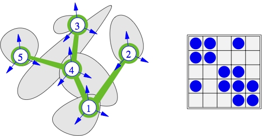
Fig. 6 A graph of local frames and the corresponding pattern of \(\mathbf{W}\).

Implementation

Local dynamics is implemented in files ldy.h and ldy.c.

Off–diagonal blocks of \(\mathbf{W}_{\alpha\beta}\) (69), diagonal block \(\mathbf{W}_{\alpha\alpha}\) (69), and the entire \(\mathbf{U}=\mathbf{B}+\mathbf{W}\mathbf{R}\) system (62) are declared in ldy.h:39 as follows:

typedef struct offb OFFB;
typedef struct diab DIAB;
typedef struct locdyn LOCDYN;

Off–diagonal blocks of \(\mathbf{W}_{\alpha\beta}\) (68) are declared in ldy.h:44 as follows:

struct offb
{
  double W [9];
  ...
  DIAB *dia;
  OFFB *n;
};

Diagonal blocks of \(\mathbf{W}_{\alpha\alpha}\) (69) and free velocity \(\mathbf{B}_{\alpha}\) (67) are declared in ldy.h:53 as follows:

struct diab
{
  double *R, /* average reaction ... */

         W [9], /* diagonal block of W */
         ...
         B [3], /* free velocity */

  OFFB *adj;

  CON *con;  /* the underlying constraint ... */

  DIAB *p, *n;

};

The local dynamics system is stored as a doubly linked list of diagonal blocs further pointing to singly linked lists of off–diagonal blocks in ldy.h:81 as:

struct locdyn
{

DIAB *dia; /* list of diagonal blocks */

};

Symbolic insertion of rows into \(\mathbf{W}\), without assembling of the numeric block values, is administered by ldy.c:LOCDYN_Insert.
Similarly, deletion of rows from \(\mathbf{W}\) is administered by ldy.c:LOCDYN_Remove.
Assembling of \(\mathbf{W}\) and \(\mathbf{B}\) is invoked by ldy.c:LOCDYN_Update_Begin.