Kinematics

A kinematic model defines an allowed type of deformation for an individual body. Solfec-1.0 includes three kinematic models:

• rigid body

• pseudo–rigid body

• finite–element body

A kinematic model is selected by specifying the kind paramter of the BODY command.

Rigid body

The motion of a rigid body reads

(12)\[\mathbf{x}\left(\mathbf{X},t\right)=\mathbf{\Lambda}\left(t\right)\left(\mathbf{X}-\bar{\mathbf{X}}\right)+\bar{\mathbf{x}}\left(t\right)\]

where \(\mathbf{\Lambda}\left(t\right)\) is a \(3\times3\) rotation matrix, \(\bar{\mathbf{X}}\) is a selected referential point, and \(\bar{\mathbf{x}}\left(t\right)\) is a spatial point. Hence \(\bar{\mathbf{x}}\left(t\right)=\mathbf{x}\left(\bar{\mathbf{X}},t\right)\) is the motion of the selected point \(\bar{\mathbf{X}}\). The term \(\mathbf{\Lambda}\left(t\right)\left(\mathbf{X}-\bar{\mathbf{X}}\right)\) represents the rotation of \(\mathbf{X}\) about the point \(\bar{\mathbf{X}}\). Representing rotations, \(\mathbf{\Lambda}\) must be orthogonal: \(\mathbf{\Lambda}^{T}\mathbf{\Lambda}=\mathbf{I}\), where \(\mathbf{I}\) is the \(3\times3\) identity matrix. Thus, the rigidity condition follows \(\left\Vert \mathbf{x}-\bar{\mathbf{x}}\right\Vert =\left\Vert \mathbf{X}-\bar{\mathbf{X}}\right\Vert\), that is the length of a line segment before and after rotation is preserved.

The velocity of the spatial point reads

(13)\[\dot{\mathbf{x}}\left(\mathbf{X},t\right)=\mathbf{\Lambda}\left(t\right)\hat{\mathbf{\Omega}}\left(t\right) \left(\mathbf{X}-\bar{\mathbf{X}}\right)+\dot{\bar{\mathbf{x}}}\left(t\right)=\hat{\mathbf{\omega}}\left(t\right) \mathbf{\Lambda}\left(t\right)\left(\mathbf{X}-\bar{\mathbf{X}}\right)+\dot{\bar{\mathbf{x}}}\left(t\right)\]

where \(\mathbf{\omega}\) is the spatial angular velocity vector, \(\mathbf{\Omega}\) is the referential angular velocity vector, and \(\dot{\bar{\mathbf{x}}}\) is the velocity of the spatial image of \(\bar{\mathbf{X}}\). W note that

\[\mathbf{\omega}=\mathbf{\Lambda}\mathbf{\Omega}\]

The hat operator \(\hat{\mathbf{y}}\) creates an anti–symmetric \(3\times3\) matrix out of a 3–vector as follows

\[\begin{split}\hat{\mathbf{y}}=\left[\begin{array}{ccc} 0 & -y_{3} & y_{2}\\ y_{3} & 0 & -y_{1}\\ -y_{2} & y_{1} & 0 \end{array}\right]\end{split}\]

In vector notation the configuration \(\mathbf{q}\) and the velocity \(\mathbf{u}\) can be expressed as

(15)\[\begin{split}\mathbf{q}=\left[\begin{array}{c} \Lambda_{11}\\ \Lambda_{21}\\ ...\\ \bar{x}_{1}\\ \bar{x}_{2}\\ \bar{x}_{3} \end{array}\right],\,\,\,\mathbf{u}=\left[\begin{array}{c} \Omega_{1}\\ \Omega_{2}\\ \Omega_{3}\\ \dot{\bar{x}}_{1}\\ \dot{\bar{x}}_{2}\\ \dot{\bar{x}}_{3} \end{array}\right]\end{split}\]

The configuration \(\mathbf{q}\) has 12 components and the velocity \(\mathbf{u}\) has 6 components.

Pseudo–rigid body

The motion of a pseudo–rigid body reads

(16)\[\mathbf{x}\left(t\right)=\mathbf{F}\left(t\right)\left(\mathbf{X}-\bar{\mathbf{X}}\right)+\bar{\mathbf{x}}\left(t\right)\]

where \(\mathbf{x}\) is the current image of a referential point \(\mathbf{X}\), \(\mathbf{F}\) is a spatially homogeneous deformation gradient \(\left(\mathbf{F}=\partial\mathbf{x}/\partial\mathbf{X}\right), \bar{\mathbf{X}}\) is a selected referential point and \(\bar{\mathbf{x}}=\bar{\mathbf{x}}\left(t\right)\) is the current image of \(\bar{\mathbf{X}}\). Deformation gradient \(\mathbf{F}\) is an invertible and orientation preserving \(\left(\det\left(\mathbf{F}\right)>0\right)\) \(3\times3\) matrix.

The velocity of the spatial point reads

(17)\[\dot{\mathbf{x}}\left(t\right)=\dot{\mathbf{F}}\left(t\right)\left(\mathbf{X}-\bar{\mathbf{X}}\right)+\dot{\bar{\mathbf{x}}}\left(t\right)\]

where \(\dot{\mathbf{F}}\) is the velocity of the deformation gradient and \(\dot{\bar{\mathbf{x}}}\) is the velocity of the spatial image of \(\bar{\mathbf{X}}\).

In vector notation the configuration \(\mathbf{q}\) and the velocity \(\mathbf{u}\) can be expressed as

(18)\[\begin{split}\mathbf{q}=\left[\begin{array}{c} F_{11}\\ F_{12}\\ ...\\ \bar{x}_{1}\\ \bar{x}_{2}\\ \bar{x}_{3} \end{array}\right],\,\,\,\mathbf{u}=\left[\begin{array}{c} \dot{F}_{11}\\ \dot{F}_{12}\\ ...\\ \dot{\bar{x}}_{1}\\ \dot{\bar{x}}_{2}\\ \dot{\bar{x}}_{3} \end{array}\right]\end{split}\]

Both, the configuration \(\mathbf{q}\) and the velocity \(\mathbf{u}\) are 12–component vectors.

Finite–element body

The finite–element motion reads

(19)\[\mathbf{x}\left(\mathbf{X},t\right)=\mathbf{X}+\mathbf{N}\left(\mathbf{X}\right)\mathbf{q}\left(t\right)\]

where \(\mathbf{x}\) is the current image of the referential point \(\mathbf{X}\), \(\mathbf{N}\left(\mathbf{X}\right)\) is a matrix of shape functions, and \(\mathbf{q}\left(t\right)\) is a vector of nodal displacements.

The velocity of the spatial point reads

(20)\[\dot{\mathbf{x}}\left(\mathbf{X},t\right)=\mathbf{N}\left(\mathbf{X}\right)\dot{\mathbf{q}}\left(t\right)\]

where \(\dot{\mathbf{q}}\) is the vector of nodal \(x,y,z\) velocities.

In vector notation, the configuration \(\mathbf{q}\) and the velocity \(\mathbf{u}\) can be expressed as

(21)\[\begin{split}\mathbf{q}=\left[\begin{array}{c} q_{1x}\\ q_{1y}\\ q_{1z}\\ ...\\ q_{nx}\\ q_{ny}\\ q_{nz} \end{array}\right],\,\,\,\mathbf{u}=\dot{\mathbf{q}}\end{split}\]

Both, the configuration \(\mathbf{q}\) and the velocity \(\mathbf{u}\) have size \(3\times n\), where \(n\) is the number of nodes in a finite–element mesh.

The matrix \(\mathbf{N}\) in (19) and (20) has the following form

\[\begin{split}\mathbf{N}=\left[\begin{array}{ccccccc} N_{1} & & & ... & N_{n}\\ & N_{1} & & ... & & N_{n}\\ & & N_{1} & ... & & & N_{n} \end{array}\right]\end{split}\]

where \(N_{i}\) are nodal shape functions, juxtaposed from element shape functions meeting at coincident mesh nodes.

Shape functions

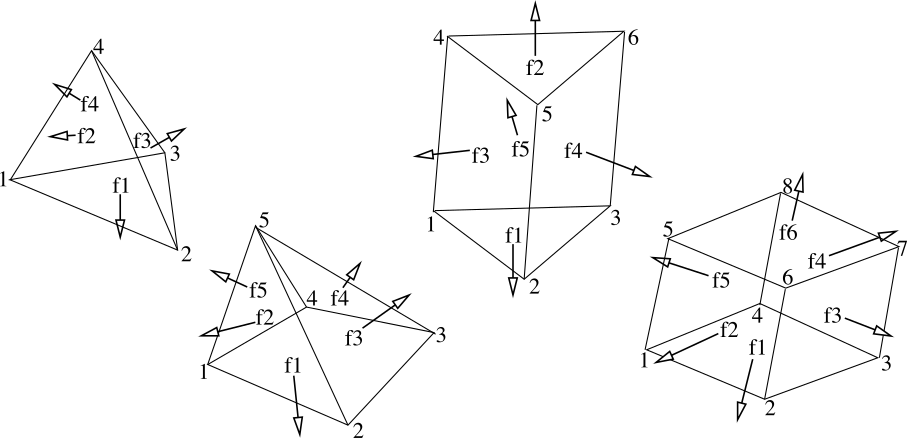
Fig. 4 Element types in Solfec-1.0: tetrahedron, pyramid, wedge, hexahedron.

Finite–element types available in Solfec-1.0 are depicted in Fig. 4. Shape functions for those elements are summarised in Table 25.

Isoparametric mapping is used to go back and forth between the natural element coordinates \(\xi_{1}\), \(\xi_{2}\), \(\xi_{3}\), local to individual element domains, and the referential mesh coordinates \(\mathbf{Y}\)

\[\begin{split}\mathbf{Y}\left(\xi_{1},\xi_{2},\xi_{3}\right)=\mathbf{N}\left(\xi_{1},\xi_{2},\xi_{3}\right)\left[\begin{array}{c} \mathbf{Y}_{1}\\ ...\\ \mathbf{Y}_{n} \end{array}\right]\end{split}\]

where \(\mathbf{Y}_{i}\) are referential coordinates of mesh nodes. The function \(\mathbf{N}\left(\mathbf{X}\right)\) in (19) and (20) has the following form

\[\mathbf{N}\left(\mathbf{X}\right)=\mathbf{N}\left(\mathbf{Y}^{-1}\left(\mathbf{X}\right)\right)\]

Newton iterations are required to solve \(\mathbf{X}=\mathbf{Y}\left(\xi_{1},\xi_{2},\xi_{3}\right)\) and find \(\xi_{1}\), \(\xi_{2}\), \(\xi_{3}\) for a given referential point \(\mathbf{X}\).

Table 25 Finite–element shape functions.

Tetrahedron

\(N_{1}=1-\left(\xi_{1}+\xi_{2}+\xi_{3}\right)\) \(N_{2}=\xi_{1}\) \(N_{3}=\xi_{2}\) \(N_{4}=\xi_{3}\)

Pyramid

\(r= \xi_{1}\xi_{2}\xi_{3}/\left(1-\xi_{3}\right)\text{ if }\xi_{3}\ne1\text{ or }0\text{ otherwise}\) \(N_{1}=0.25\left(\left(1+\xi_{1}\right)\left(1+\xi_{2}\right)-\xi_{3}+r\right)\) \(N_{2}=0.25\left(\left(1-\xi_{1}\right)\left(1+\xi_{2}\right)-\xi_{3}-r\right)\) \(N_{3}=0.25\left(\left(1-\xi_{1}\right)\left(1-\xi_{2}\right)-\xi_{3}+r\right)\) \(N_{4}=0.25\left(\left(1+\xi_{1}\right)\left(1-\xi_{2}\right)-\xi_{3}-r\right)\) \(N_{5}=\xi_{3}\)

Wedge

\(N_{1}=0.5\left(1-\xi_{1}-\xi_{2}\right)\left(1-\xi_{3}\right)\) \(N_{2}=0.5\xi_{1}\left(1-\xi_{3}\right)\) \(N_{3}=0.5\xi_{2}\left(1-\xi_{3}\right)\) \(N_{4}=0.5\left(1-\xi_{1}-\xi_{2}\right)\left(1+\xi_{3}\right)\) \(N_{5}=0.5\xi_{1}\left(1+\xi_{3}\right)\) \(N_{6}=0.5\xi_{2}\left(1+\xi_{3}\right)\)

Hexahedron

\(N_{1}=0.125\left(1-\xi_{1}\right)\left(1-\xi_{2}\right)\left(1-\xi_{3}\right)\) \(N_{2}=0.125\left(1+\xi_{1}\right)\left(1-\xi_{2}\right)\left(1-\xi_{3}\right)\) \(N_{3}=0.125\left(1+\xi_{1}\right)\left(1+\xi_{2}\right)\left(1-\xi_{3}\right)\) \(N_{4}=0.125\left(1-\xi_{1}\right)\left(1+\xi_{2}\right)\left(1-\xi_{3}\right)\) \(N_{5}=0.125\left(1-\xi_{1}\right)\left(1-\xi_{2}\right)\left(1+\xi_{3}\right)\) \(N_{6}=0.125\left(1+\xi_{1}\right)\left(1-\xi_{2}\right)\left(1+\xi_{3}\right)\) \(N_{7}=0.125\left(1+\xi_{1}\right)\left(1+\xi_{2}\right)\left(1+\xi_{3}\right)\) \(N_{8}=0.125\left(1-\xi_{1}\right)\left(1+\xi_{2}\right)\left(1+\xi_{3}\right)\)

Implementation

Kinematic models are implement in bod.c (rigid, pseudo–rigid) and fem.c (finite–element) files. Configuration and velocity vectors are declared in bod.h as follows:

struct general_body
{
  enum {OBS, RIG, PRB, FEM} kind; /* obstacle, rigid, pseudo-rigid, finite element */

  /* ... */

  double *conf,    /* configuration */
         *velo;    /* velocity */

  /* ... */
}