Constraints

Constraints allow to limit kinematic freedom of bodies, e.g. control displacements or prevent interpenetration. This is reflected on the level of dynamics via reaction forces, which are used to produce desired kinematic effects. Solfec-1.0 includes equality constraints, or joints, and contact constraints applied at individual contact points. In this section we briefly demonstrate how constraints are incorporated into the time stepping schemes introduced earlier.

From global to local velocity

Velocity \(\mathbf{u}\), as defined for rigid, pseudo-rigid, and finite–element bodies, can be qualified as a global, or generalized, or bodytextendash space entity. In order to obtain a local, spatial 3–dimensional velocity vector, \(\mathbf{U}\), of any spatial image \(\mathbf{x}\) of a referential point \(\mathbf{X}\), we shall use a linear transformation of the kind

(44)\[\mathbf{U}=\mathbf{H}\left(\mathbf{X}\right)\mathbf{u}\]

Most generally the local velocity \(\mathbf{U}\) will be expressed in a local coordinate system, made up of three linearly independent 3–vectors, \(\mathbf{a}_{i}\), juxtaposed, in a column–wise manner into a matrix \(\left\{ \mathbf{a}_{i}\right\}\), also called local frame, cf. Fig. 5. Such matrix will have an inverse which we can denote as \(\left\{ \mathbf{a}^{i}\right\} ^{T}=\left\{ \mathbf{a}_{i}\right\} ^{-1}\). The two coordinate systems, \(\left\{ \mathbf{a}_{i}\right\}\) and \(\left\{ \mathbf{a}^{i}\right\}\), are traditionally referred to as covariant and contravariant, respectively. In Solfec-1.0 we use an orthogonal local base \(\left\{ \mathbf{a}_{i}\right\}\) and in this case \(\left\{ \mathbf{a}^{i}\right\} =\left\{ \mathbf{a}_{i}\right\}\), so that \(\left\{ \mathbf{a}^{i}\right\} ^{T}=\left\{ \mathbf{a}_{i}\right\} ^{T}\). Consequently, the local frame is functionally equivalent to a rotation matrix.

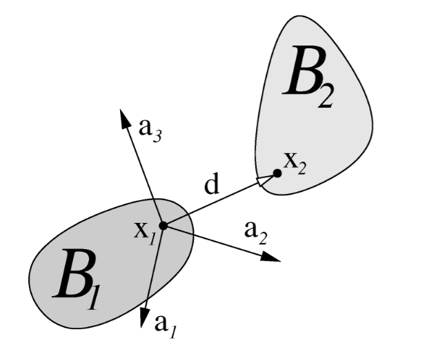
Fig. 5 A local frame between two bodies.

The linear transformation (44) can be most generally derived as follows. Take any motion

\[\mathbf{x}\left(\mathbf{X},t\right)=\chi\left(\mathbf{X},\mathbf{q}\left(t\right)\right)\]

and calculate its derivative with respect to time

\[\dot{\mathbf{x}}\left(\mathbf{X},t\right)=\frac{\partial\chi\left(\mathbf{X},\mathbf{q}\left(t\right)\right)}{\partial\mathbf{q}}\mathbf{u}\left(t\right)\]

Then transform this spatial velocity from the global Euclidean frame into the local frame

\[\mathbf{U}=\left\{ \mathbf{a}^{i}\right\} ^{T}\frac{\partial\chi\left(\mathbf{X},\mathbf{q}\left(t\right)\right)}{\partial\mathbf{q}}\mathbf{u}\]

Thus

(45)\[\mathbf{H}\left(\mathbf{X}\right)=\left\{ \mathbf{a}^{i}\right\} ^{T}\frac{\partial\chi\left(\mathbf{X},\mathbf{q}\left(t\right)\right)}{\partial\mathbf{q}}\]

Specific forms of this transformation are described in sections below.

Rigid kinematics

For rigid bodies, there holds

\[\dot{\mathbf{x}}=\mathbf{\Lambda}\hat{\mathbf{\Omega}}\left(\mathbf{X}-\bar{\mathbf{X}}\right)+\dot{\bar{\mathbf{x}}}\]

\[\begin{split}\mathbf{u}=\left[\begin{array}{c} \mathbf{\Omega}\\ \dot{\bar{\mathbf{x}}} \end{array}\right]\end{split}\]

and hence

(46)\[\mathbf{H}=\left\{ \mathbf{a}^{i}\right\} ^{T}\left[\begin{array}{ccc} \mathbf{\Lambda}\left(\hat{\bar{\mathbf{X}}}-\hat{\mathbf{X}}\right) & & \mathbf{I}\end{array}\right]\]

where the hat operator makes an anti–symmetric matrix out of a 3–vector, and \(\mathbf{I}\) is a \(3\times3\) identity matrix.

Pseudo–rigid kinematics

For pseudo-rigid bodies, there holds

\[\dot{\mathbf{x}}=\dot{\mathbf{F}}\left(\mathbf{X}-\bar{\mathbf{X}}\right)+\dot{\bar{\mathbf{x}}}\]

\[\begin{split}\mathbf{u}=\left[\begin{array}{c} \dot{F}_{11}\\ \dot{F}_{12}\\ ...\\ \dot{\bar{\mathbf{x}}} \end{array}\right]\end{split}\]

and hence

(47)\[\begin{split}\mathbf{H}=\left\{ \mathbf{a}^{i}\right\} ^{T}\left[\begin{array}{cccccc} \mathbf{X}^{T}-\bar{\mathbf{X}}^{T} & & & 1\\ & \mathbf{X}^{T}-\bar{\mathbf{X}}^{T} & & & 1\\ & & \mathbf{X}^{T}-\bar{\mathbf{X}}^{T} & & & 1 \end{array}\right]\end{split}\]

Finite–element kinematics

For finite–element bodies, there holds

\[\dot{\mathbf{x}}\left(\mathbf{X},t\right)=\mathbf{N}\left(\mathbf{X}\right)\mathbf{u}\]

and hence

(48)\[\mathbf{H}=\left\{ \mathbf{a}^{i}\right\} ^{T}\mathbf{N}\left(\mathbf{X}\right)\]

Time stepping with constraints

If we wish to control components of a local velocity \(\mathbf{U}\) at a point \(\mathbf{x}\), we can do this by applying a force \(\mathbf{R}\) at this point. Such local force \(\mathbf{R}\) is reflected as a global, or generalized, or body–space force, \(\mathbf{r}\) as follows

\[\mathbf{r}=\mathbf{H}^{T}\mathbf{R}\]

The momentum balance is modified accordingly

\[\mathbf{M}\dot{\mathbf{u}}=\mathbf{f}+\mathbf{H}^{T}\mathbf{R}\]

In case of multiple forces, \(\mathbf{R}_{\alpha}\), applied at multiple points \(\mathbf{x}_{\alpha}\), and controlling multiple local velocities \(\mathbf{U}_{\alpha}\), the modified momentum balance reads

\[\mathbf{M}\dot{\mathbf{u}}=\mathbf{f}+\sum_{\alpha}\mathbf{H}_{\alpha}^{T}\mathbf{R}_{\alpha}\]

Our attempt to control components of local velocities can be interpreted as applying constraints. With such understanding, we can call \(\mathbf{U}_{\alpha}\) constraints velocities, and \(\mathbf{R}_{\alpha}\) constraints reactions. For the sake of convenience, in case of a multi–body system, we can use symbols \(\mathbf{M}\), \(\mathbf{q}\), \(\mathbf{u}\), \(\mathbf{f}\), \(\mathbf{H}\), \(\mathbf{U}\), \(\mathbf{R}\), etc. as suitably juxtaposing matrices and vectors of all associated individual bodies or constraints. For example

\[\begin{split}\mathbf{U}=\left[\begin{array}{c} ...\\ \mathbf{U}_{\alpha}\\ ... \end{array}\right],\,\,\,\mathbf{R}=\left[\begin{array}{c} ...\\ \mathbf{R}_{\alpha}\\ ... \end{array}\right]\end{split}\]

\[\mathbf{H}=\left[\begin{array}{ccc} ... & \mathbf{H}_{\alpha} & ...\end{array}\right]\]

\[\begin{split}\mathbf{M}=\left[\begin{array}{ccc} ...\\ & \mathbf{M}_{i}\\ & & ... \end{array}\right],\,\,\,\mathbf{f}=\left[\begin{array}{c} ...\\ \mathbf{f}_{i}\\ ... \end{array}\right],\,\,\,\mathbf{u}=\left[\begin{array}{c} ...\\ \mathbf{u}_{i}\\ ... \end{array}\right]\end{split}\]

With such understanding in mind, we can incorporate any set of constraints into a multi–body system, by saying

(49)\[\mathbf{M}\dot{\mathbf{u}}=\mathbf{f}+\mathbf{H}^{T}\mathbf{R}\]

(50)\[\mathbf{U}=\mathbf{H}\mathbf{u}\]

(51)\[\mathbf{C}\left(\mathbf{U},\mathbf{R}\right)=\mathbf{0}\]

where the relation \(\mathbf{C}\left(\mathbf{U},\mathbf{R}\right)=\mathbf{0}\) implicitly expresses a control over local velocities \(\mathbf{U}_{\alpha}\), exerted using reaction forces \(\mathbf{R}_{\alpha}\). Now, including constraints, we can modify the previously introduced time stepping as follows

(52)\[\mathbf{q}^{t+\frac{h}{2}}=\mathbf{q}^{t}+\frac{h}{2}\mathbf{u}^{t}\]

(53)\[\mathbf{u}^{t+h}=\mathbf{u}^{t}+\mathbf{A}^{-1}h\mathbf{f}\left(\mathbf{q}^{t+\frac{h}{2}},\mathbf{u}^{t}\right)+ \mathbf{A}^{-1}h\mathbf{H}^{T}\left(\mathbf{q}^{t+\frac{h}{2}}\right)\mathbf{R}\]

(54)\[\mathbf{U}=\mathbf{H}\left(\mathbf{q}^{t+\frac{h}{2}}\right)\mathbf{u}\]

(55)\[\mathbf{C}\left(\mathbf{U},\mathbf{R}\right)=\mathbf{0}\label{eq:CUR2}\]

(56)\[\mathbf{q}^{t+h}=\mathbf{q}^{t+\frac{h}{2}}+\frac{h}{2}\mathbf{u}^{t+h}\]

The first step (57) is explicit. Equations (58), (59), (60) are solved together, implicitly. The final step (61) is again explicit. This form of constrained time integration is implemented in Solfec-1.0.

Implementation

Calculation of the global to local velocity mapping \(\mathbf{H}\) is implement in bod.c (rigid, pseudo–rigid) and fem.c (finite–element) files. A constraint data structure, including the local frame \(\left\{ \mathbf{a}_{i}\right\}\), the spatial point \(\mathbf{x}\), the constraint velocity \(\mathbf{U}\), and rection \(\mathbf{R}\), is declared in dom.h as follows:

#define VELODIR1(Z)     ((Z)[1])   /* prescribed velocity at (t+h) */
#define VELODIR2(Z)     ((Z)[2])   /* prescribed velocity at (t+h) */

enum constraint_state
     {CON_COHESIVE = 0x01,
      CON_NEW      = 0x02,  /* newly inserted constraint */
      CON_IDLOCK   = 0x04,  /* locked ID cannot be freed to the pool */
      CON_EXTERNAL = 0x08,  /* a boundary constraint migrated in from another processor */
      CON_DONE     = 0x10}; /* auxiliary flag used in several places */

struct constraint
{

  /* put parallel data at the end of the structutre so that

Evaluation of (45) in accessed via bod.c:BODY_Gen_To_Loc_Operator.
Assembling of (46) is in bod.c:rig_operator_H.
Assembling of (47) is in bod.c:prb_operator_H.
Assembling of (48) is in fem.c:FEM_Gen_To_Loc_Operator.