Masonry arch

Reference: Gilbert, M. and Casapulla, C. and Ahmed, H. M., Limit analysis of masonry block structures with non-associative frictional joints using linear programming, Computers and Structures, vol. 84, pp. 873-887, 2006. Analysis: Explicit dynamics, frictional contact. Purpose: Examine applicability of the dynamic scheme to the limit-state analysis of frictional block structures. Summary: A semicircular arch is composed of 27 blocks, subjected to the uniform gravitational field. The dynamic stability of the arch is investigated for varying ratios of the thickness to centreline radius \(h/r\). The results are compared against the available findings based on the limit-state analysis.

Gilbert et al. 1 present a numerical solution to the classical problem of the stability of a semicircular arch under gravity load. The analysis provided in 1 spans friction coefficients from the interval \(\left[0.2,0.8\right]\) and identifies three geometrical failure modes (Fig. 26). The classical analysis provided by Heyman 2 assumes no frictional slip, and therefore covers only one case of mechanism formation (mode I – typical for large friction).

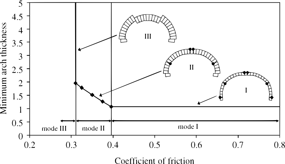
Fig. 26 Symmetrical arch problem: influence of friction coefficient on minimum arch thickness (after Gilbert et al. 1).

Several factors need to be taken into account when considering reproduction of the results presented in Fig. 26:

1. A linear programming based limit–state formulation is employed in 1, whereas the dynamic contact algorithm is used in Solfec-1.0.

2. The analysis provided in 1 is two–dimensional, whereas Solfec-1.0 deals with a three–dimensional model.

3. A node to face contact model is employed in 1, whereas the face to face (or more generally element to element) contact model is employed in Solfec-1.0.

Due to the modeling differences (inertial effects, contact resolution) is it reasonable to accept a margin of discrepancy between the results obtained by both methods. The dynamic stability analysis will be based on the observation of the kinetic energy histories, calculated for arches with thicknesses varying around the documented in 1 stability limits. Fig. 27 summarizes the geometry and discretization adopted in the Solfec-1.0 model. In order to geometrically capture the hinging effect from the first moments of simulation, the subdivision along the block thickness comprises two narrow elements at the extrados and intrados of the arch.

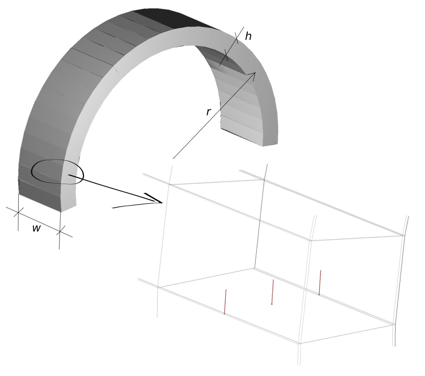
Fig. 27 The three–dimensional arch model in Solfec-1.0. Each of the 27 blocks is composed of 6 elements: two along the width \(w\), and three along the thickness \(h\). Thus six contact points are established initially between a pair of blocks.

Input parameters

Under the assumptions discussed by Heyman 2, formation of a failure mechanism is of purely geometrical nature. Therefore the material parameters can be chosen arbitrary (none have been reported in 1). The table below summarizes the assumed parameters.

Mass density \(\left(kg/m^{3}\right)\)	\(\rho=1\)
Centreline radius \(\left(m\right)\)	\(r=10\)
Arch width \(\left(m\right)\)	\(w=5\)
Number of blocks	27
Initial velocities \(\left(m/s\right)\)	all zero
Gravity acceleration \(\left(m/s^{2}\right)\)	\(\mathbf{g}=\left[0,0,-9.81\right]\)
Velocity restitution	\(\epsilon=0\)
Time step \(\left(s\right)\)	\(h=0.001\)
Simulated duration \(\left(s\right)\)	\(0.1\)

Results

Fig. 28 illustrates the kinetic energy of the arch model at the end of the 0.1s simulated duration. A range of values of the coefficient of friction and arch thickness to radius ratios \(h/r\) was used. The region above the 0.001–level contour line corresponds to the “numerical zero” level of kinetic energy, where the arch remains stable. For the parameters below this level curve the arch begins to collapse.

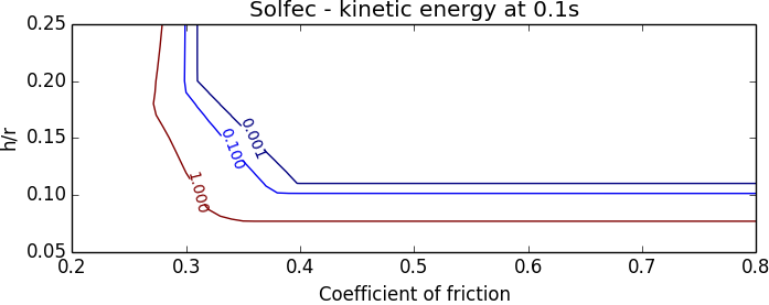
Fig. 28 Kinetic energy map at the end of the 0.1s simulations over a grid of friction coefficients and \(h/r\) ratios.

Fig. 29 superimposes Fig. 26 from [1] with Fig. 28. We can see that the transition lines coincide. Fig. 29 also includes the failure modes I, II, and III reproduced from three longer Solfec-1.0 simulations (to allow for more deformation). It is seen that the six–hinge mechanism is exactly formed for large friction (mode I). The mode II mechanism is qualitatively well captured in Fig. 29. The four–hinge mechanism does form in the initial phase of the dynamic solution, yet, due to the sensitivity of the dynamic simulation, one of the top hinges “takes over” at a later stage (no deformation scaling was applied in the figures). Also the the qualitative nature of mode III deformation in Fig. 29 reflects the corresponding mode in Fig. 26. Small differences owe to the modeling discrepancies.

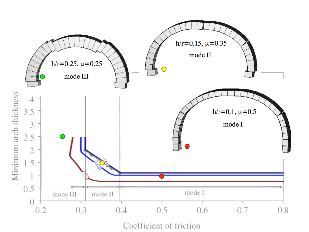
Fig. 29 Level curves from Fig. 28 obtained from Solfec-1.0 superimposed with Fig. 26 from [1]. The corresponding three modeled failure modes are included.

1(1,2,3,4,5,6,7,8)

Gilbert, M. and Casapulla, C. and Ahmed, H. M., Limit analysis of masonry block structures with non-associative frictional joints using linear programming, Computers and Structures, vol. 84, pp. 873-887, 2006.

2(1,2)

Heyman, Jacques, “Equilibrium of Shell Structures”, Clarendon Press (1977).