Pendulum

Reference: W. Rubinowicz, W. Królikowski, Mechanika teoretyczna (Theoretical mechanics), Państwowe Wydawnictwo Naukowe, Warszawa, 1998, pp. 91-99. Analysis: Explicit dynamics, bilaterally constrained motion. Purpose: Examine the accuracy of an analysis involving rigid rod constraint. Summary: A mathematical pendulum composed of a mass point and a weightless rod swings with a large amplitude. Pendulum period, energy conservation, constraint satisfaction and convergence are examined.

The period of an oscillatory mathematical pendulum reads

\[T=2\pi\sqrt{\frac{l}{g_{3}}}\left(1+\left(\frac{1}{2}\right)^{2}k^{2}+\left(\frac{1\cdot3} {2\cdot4}\right)k^{2}+\left(\frac{1\cdot3\cdot5}{2\cdot4\cdot6}\right)k^{2}+...\right)\]

where

\[k=\sin\left(\frac{\theta_{max}}{2}\right)\]

and \(l\) is the length of the pendulum, \(g_{3}\) is the vertical component of the gravity acceleration and \(\theta_{max}\) is the maximal tilt angle of the pendulum. Let us assume the initial velocity of the pendulum to be zero. Thus \(\theta_{max}=\theta\left(0\right)\). Taking the rest configuration position of the mass point \(\bar{\mathbf{x}}=\left[0,0,0\right]\) and considering the swing in the \(x-z\) plane, the initial position of the pendulum reads

\[\begin{split}\bar{\mathbf{x}}\left(0\right)=\left[\begin{array}{c} l\sin\left(\theta_{max}\right)\\ 0\\ l\left(1-\cos\left(\theta_{max}\right)\right) \end{array}\right]\end{split}\]

Without the initial kinetic energy \((E_{k}\left(0\right)=0)\), the energy conservation requires that

\[E_{k}\left(t\right)+E_{p}\left(t\right)=E_{p}\left(0\right)\]

where

\[E_{p}\left(0\right)=mg_{3}\bar{x}_{3}\left(0\right)\]

and \(m\) is the scalar mass.

Input parameters

Length \(\left(m\right)\)	\(l=1\)
Mass \(\left(kg\right)\)	\(m=1\)
Initial angle \(\theta\left(0\right)=\theta_{max}\,\, \left(rad\right)\)	\(\theta_{max}=\pi/2\)
Gravity acceleration \(\left(m/s^{2}\right)\)	\(\mathbf{g}=\left[0,0,-\pi^{2}\right]\)

The gravity acceleration \(g_{3}\) has been chosen so that for \(\theta_{max}=0\deg\) there holds \(T=2s\).

Results

The table below summarizes the results for the time step \(h=0.001\). The solution is accurate and stable after 1 and 10 swings. Fig. 17 illustrates the energy balance over one period of the pendulum. The potential and kinetic energies sum up to \(\pi^{2}\).

	Target	Solfec-1.0	Ratio
Pendulum period – 1 swing \(\left(s\right)\)	2.360	2.360	1.000
Total energy – 1 swing \(\left(J\right)\)	\(\pi^{2}\)	9.86960	1.000
Pendulum period – 10 swings \(\left(s\right)\)	23.60	23.60	1.000
Total energy – 10 swings \(\left(J\right)\)	\(\pi^{2}\)	9.86960	1.000

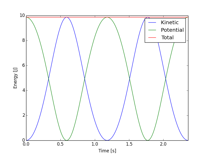
Fig. 17 Energy balance over one period of the pendulum.